Building a Recurrent Neural Network from Scratch with Python and Mathematics

Photo by Thorium

Following my ML Learning Path, after learning and implementing Linear Regression, Logistic Regression, Neural Network, and Deep Neural Network, it's time to learn about sequence problems and how Recurrent Neural Networks (RNNs) handle these kinds of challenges.

In this post, we will follow the same recipe as the previous posts in this series: work on the theory behind the ML model, give an overview of how mathematics shapes it, and implement everything from scratch using Python and NumPy.

Here are the topics I'm going to cover:

• Sequence Problems & How RNNs Fit Them
• Types of Problems for RNNs
• RNN Theory & Math
• Vanishing/Exploding Gradients Problem
• Implementing From Scratch

Let's start!

Sequence Problems & How RNNs Fit Them

Many sequence problems can be modeled by machine learning. These kinds of problems show up in many life situations. The financial market is a classic example of sequence data. Another one is weather forecasting.

The fundamental idea behind sequence problems is that they have temporal dependency. To predict the future, we need to understand both the past and the present. Previous observations define a sequence problem.

Standard Neural Networks have limitations when it comes to sequence problems. They require a fixed input size. These kinds of networks don't have a dynamic adjustment for the number of input neurons or the dimensions of the weight matrices based on the input's size.

For example, if you train a standard neural network to classify images that are 28x28 pixels (784 pixels flattened into a vector), its input layer will have 784 neurons. You cannot then feed it a 32x32 pixel image (1024 pixels) without reshaping it or altering the network's architecture. The number of input and neurons are fixed.

For sequence problems, inputs and outputs can have different sizes for different examples. As we will see, it behaves like it has many feedforward neural nets.

Another big limitation of standard neural networks is regarding the underlying characteristic of sequence problems: temporal dependency.

Standard neural networks don't share their learned parameters across different input positions. For sequence data, it's crucial to utilize information derived from previous positions when computing current ones.

Recurrent Neural Networks handle these two challenges. They overcome the temporal dependency limitation by introducing the concept of a recurrent connection and parameter sharing across time steps. Because they can process sequence data one element (or one time step) at a time, they can have different input sizes and variable output.

Types of Problems for RNNs

As we learned in the previous section, Recurrent Neural Networks (RNNs) are particularly well-suited for tasks involving sequence problems. Their ability to process sequences makes them effective in different types of applications.

These types fall into 3 categories: Many-to-One, One-to-Many, and Many-to-Many.

In Many-to-One applications, we have Sequence-to-Vector tasks. In this setup, an RNN takes a sequence of inputs and produces a single output. These are some of the examples:

• Spam detection: The content of an email (a sequence of words) is fed into the RNN. The network accumulates information and context from the words and outputs a binary classification to predict whether the email is spam or not.
• Sentiment analysis: It tries to predict the emotional tone of a text. Based on a sequence of words, the RNN classifies whether the text has positive, negative, or neutral sentiment.
• Weather forecasting: RNNs can also be used for single-point weather forecasting, taking a sequence of past weather data to predict tomorrow's weather.

In One-to-Many applications, we have Vector-to-Sequence tasks. It takes a single input and generates a sequence as output. Image captioning is the classic example of this. An image is processed by the RNN, and the model generates a caption (a sequence of words). The previous parameters and predicted words serve as input to predict the subsequent word, building the caption text.

The most sophisticated category is the Many-to-Many applications, where we have Sequence-to-Sequence tasks (Seq2Seq). Machine translation is the most famous example here. A sentence in one language (an input sequence of words) is translated into a sentence in another language (an output sequence of words). This is typically achieved using an RNN Encoder-Decoder architecture.

• The encoder RNN processes the input sequence, effectively "understanding" the language and context, and compresses this information to be used as input.
• The decoder RNN then takes this encoded information and generates the new language text, token by token, building the translated output sequence.

RNN Theory & Math

In this section, we'll dive into the theory and math behind Recurrent Neural Networks. This is one of the most interesting concepts I have studied so far, as it combines the ideas of standard neural networks with a recurrent mechanism so it can memorize and reuse the learned parameters from the past to predict the future.

If I could tell anyone about RNNs, I would say exactly that. It's a standard neural network together with a recurrent mechanism. But what does that mean? We need to dive into these two ideas: standard neural networks and the recurrent mechanism.

A standard neural network uses the concepts of layers. The input layer, the hidden layers, and the output layer.

In the hidden layers, it applies non-linear functions called activation functions.

In the output layer, it will make the prediction. If it's a classification problem, it will probably be something similar to cross-entropy to compute the probabilities of each class, and a linear activation function for regression problems (together with MSE to compute the loss).

This is the same idea behind RNNs. The new concept here is the recurrent mechanism.

The architecture of RNNs has a sequence of layers:

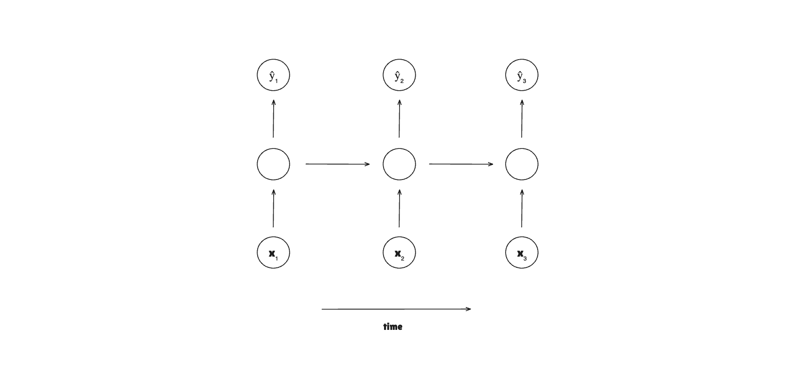
For each sequence item, it will run the standard neural network with the ”memory”. Each item in the sequence is called a time step.

The recurrent mechanism handles the “memory” by storing hidden states and passing them through each time step. Each time step receives the hidden state of the previous time step, so it can use the learned parameters from previous steps.

In summary, it receives an input, the previous hidden state, computes a linear combination, and applies an activation function to produce a new hidden state that will be passed to the next time step.

These hidden states are parameters that are shared across time. Each time step can output a probability (classification) or a scalar value (regression).

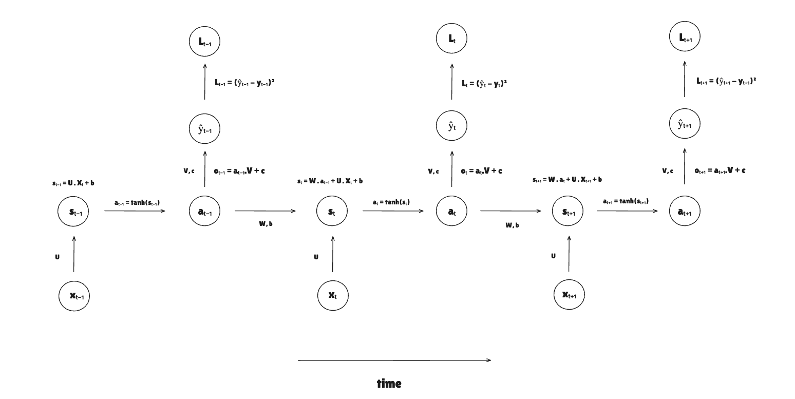
Here are all the parameters and variables used in this RNN:

• $U$: input weight
• $W$: activation weight
• $b$: bias for the weighted sum
• $a_{t-1}$: activation from previous time step (hidden state)
• $s_t$: hidden layer weighted sum
• $a_t$: activation from the current time step
• $V$: output weight
• $c$: bias for output weighted sum
• $o_t$: prediction output

Similar to how the predictions are calculated layer by layer through time steps in the forward pass, we compute the gradients in reverse order, backwards through time.

In backpropagation through time, we need to calculate the gradients all the way from the loss function to the parameters used in each layer and then pass “shared” gradients to the previous steps.

The idea of backpropagation is to make the model learn, meaning it should update the parameters based on the loss function. To update the parameters, we need the gradients for each parameter. As we will see, to compute the gradients for the parameters, we need to compute everything from the ground up.

We start from the loss function of the last time step and compute its gradient. In the problem we'll see in this post, the loss function used will be the Mean Squared Error (MSE) loss function.

The equation for this loss function is the following:

We first compute the derivative of the loss function with respect to the output: ${\frac{\partial L_t}{\partial o_t}}$.

We want to find how the loss changes with respect to a change in a single element ${o_t}$ of the output ${o}$. We can use the chain rule:

In the output layer, we can now compute the gradients for the $V$ (output weight parameter) and $c$ (bias) parameters using the chain rule.

For the $c$ gradient, we have:

We know that $\frac{\partial L}{\partial o_t} = \hat{y}_t - y_t$, so we just need to compute $\frac{\partial o_t}{\partial c}$.

Putting everything together, we have:

$V$ gradient follows the same idea.

Again, $\frac{\partial L_t}{\partial o_t} = y_t - \hat{y}_t$, so we just miss the calculation of $\frac{\partial o_t}{\partial V}$

Putting everything together, we have:

With that, we finish the computation of gradients for the output layer. With those gradients, we can reuse them in the computation of gradients in the hidden layer.

In the hidden layer, the idea is to compute the gradients for $W$ and $b$. That way, we can update these parameters in the backpropagation and make the model learn.

To reach these gradients, we first need to compute the derivative of the loss with respect to the current activation, then reuse this value to compute the gradient for the weighted sum of the current time step. With those values, we can compute the gradients for $W$ and $b$.

Let's start with the current activation. This is an important step as it requires two steps.

1. Computing the gradient of the current step activation with respect to the current output
2. Computing the gradient of the current step activation with respect to the next step's loss

To calculate the whole $\frac{\partial L_t}{\partial a_t}$, we need to compute these two steps and then sum them.

Starting with the gradient of the current activation with respect to the current output, we have:

From the previous computations, we know that

So we only miss the calculation of $\frac{\partial L_t}{\partial a_t}$ :

Putting everything together, we have:

For $\frac{\partial L_{t+1}}{\partial a_t}$, we have:

For $\frac{\partial s_{t+1}}{a_t}$, we have:

Putting everything together to compute the gradient of the loss with respect to the current activation, we have:

We can now proceed with the gradient for the weighted sum of the current time step.

Here, we need to compute the derivative of the loss with respect to the weighted sum $\frac{\partial L_t}{\partial s_t}$.

$\frac{\partial L_t}{\partial a_t}$ is what we computed previously. $\frac{\partial a_t}{\partial s_t}$ is what is missing.

Putting everything together, we have:

With both $\frac{\partial L_{t}}{a_t}$ and $\frac{\partial L_t}{\partial s_t}$, we can now compute the gradients of $W$ and $b$.

For $W$, we can simplify it:

We do a similar calculation for $b$. Given that:

We have:

In the input layer, we also need to compute the gradient of $U$.

To complete the computation of gradients, we need to do the full backpropagation. Basically, we compute the gradients for all time steps. And only after that, we can use their value to update the parameters.

These are the parameters we need to update to make the RNN model learn:

This is the full backpropagation.

Vanishing/Exploding Gradients Problem

Before moving on to the implementation section, let's talk very briefly about the vanishing and exploding gradients problem.

With deep layers and long sequences, the gradients have a very hard time propagating back to affect the weights in RNNs.

This happens because the gradients at earlier time steps are computed by multiplying the gradients from later time steps.

If the values in the weight matrices or the derivatives of the activation functions are consistently less than 1, then with each multiplication through the time steps, the gradient becomes progressively smaller over time, turning that into a vanishing gradient problem.

This is a very common deep learning problem because activation functions contribute to the shrinking gradient problem. They have derivatives that are always less than or equal to 1.

For the exploding gradient problem, it's the opposite. It becomes too big. We usually see "NaN" (numerical overflow) values, and it is easier to spot the problem.

In this post, we will focus on the internal work of RNNs and not on the vanishing/exploding gradients problem. In future posts, I plan to write about GRU and LSTM, which are more sophisticated types of RNN that handle this limitation of simple RNNs.

But I wanted to give you a brief overview of this common problem in deep learning, before moving on to the implementation part, and let you know that this implementation could lead to this problem.

Implementing From Scratch

The motivation problem for this implementation will be an arithmetic sequence prediction. The RNN will be tasked with learning the underlying rule (the common difference) of an arithmetic sequence so that, given a sequence, it can predict the subsequent numbers.

For example, for this sequence [1, 3, 5, 7, 9], the common difference is 2. So the expected output should be [3, 5, 7, 9, 11].

• For input 1, the target is 3.
• For input 3, the target is 5.
• For input 5, the target is 7.
• For input 7, the target is 9.
• For input 9, the target is 11 (which is 9 + 2).

Let's generate the data to train the model.

def generate_arithmetic_sequence_data(number_of_sequences, sequence_length, max_start=10, max_diff=5):
    X_data = []
    Y_data = []

    for _ in range(number_of_sequences):
        start_value = np.random.randint(1, max_start)
        diff = np.random.randint(1, max_diff)
        sequence = [start_value + i * diff for i in range(sequence_length + 1)]
        X_data.append(np.array(sequence[:-1]).reshape(sequence_length, 1))
        Y_data.append(np.array(sequence[1:]).reshape(sequence_length, 1))

    return np.array(X_data), np.array(Y_data)

The idea here is to programmatically generate sequences for this arithmetic problem. We pass the number of sequences we need for this training and the function will figure that out.

The starting number and the common difference are generated randomly using np.random.randint.

Notice that we can also pass max_start and max_diff to the function. That will help control the generated input data. For our first experiments, we don't want a huge common difference.

After generating this sequence, we select the first n - 1 numbers as the $X$ input, n being the sequence length. The Y target is basically the sequence from 1 to n.

X_data and Y_data are the vectors of sequences and targets.

Moving on, let's talk briefly about the architecture of this implementation.

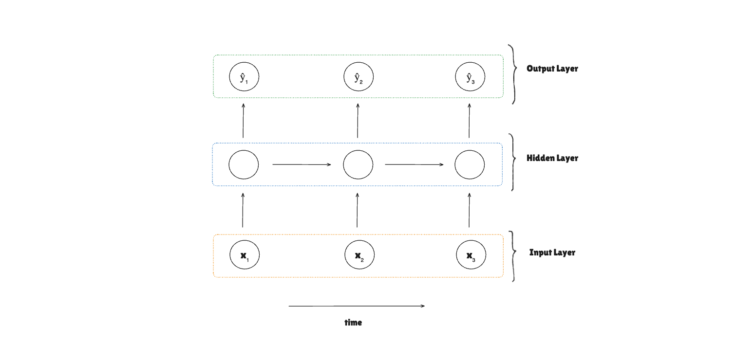
We'll have 4 parts:

• Input Layer: It will receive the input sequence, compute the input weighted sum in the forward pass, and compute the gradients in the backpropagation to update the input weight parameter $U$.
• Hidden Layer: It computes the activation and stores it in the hidden state, which will be carried on through the RNN. It computes the gradients for $W$ and bias $b$, and updates these parameters and propagates the gradients to the previous time step.
• Output Layer: It computes the prediction and the gradients for output parameters $V$ and bias $c$, and the output gradient to pass back to the hidden layer, and updates the parameters.
• RNN: It puts everything together — forward propagation, backward propagation, training with epochs, and loss function with MSE.

Let's go to the implementation, finally.

How is it going to work? First, we will do the forward pass, from the input layer to the hidden layer, and finally the output layer. And then do backpropagation through time, from output to input layer, computing all the gradients and updating the parameters.

Then, put everything together on the RNN abstraction class. And finally, use it to train the arithmetic data we generated previously and make predictions.

Forward Propagation

Everything starts in the input layer. For the forward propagation, we need two things: to initialize the parameters and compute the weighted sum.

In the __init__ method, we start with the $U$ weight parameter and the input_sequence.

class InputLayer:
    def __init__(self, input_features_size, hidden_size):
        self.U = xavier_uniform(input_features_size, hidden_size)
        self.input_sequence = None

Let's unwrap this implementation. input_sequence starts with a nullable value. For each time step, we will set the item of the sequence and then compute the weighted sum.

For the $U$ weight parameter, we can initialize it with random numbers or even with zeros. Vanishing/exploding gradients are a big problem in neural networks. Especially in RNN, this is an even bigger problem. We will use the Xavier initialization to mitigate this problem with the aim of preventing activations from becoming too small or too large.

def xavier_uniform(fan_in, fan_out):
    limit = np.sqrt(6 / (fan_in + fan_out))
    return np.random.uniform(-limit, limit, size=(fan_out, fan_in))

We also implement a getter and setter for the input sequence.

def get_input(self, time_step):
    return self.input_sequence[time_step].reshape(-1, 1)

def set_input(self, input_sequence):
    self.input_sequence = input_sequence

The setter is simple. Just pass the input_sequence and store it in the instance so we can reuse it in weighted sum and other operations.

For the getter method, we need to perform a simple transformation on the sequence data. First, it should receive the time step, so we get the correct input in the sequence. Then, we perform the transformation.

The shape of self.input_sequence is (5, 1). If we get the input of the current time step, the shape will be (1,). We use reshape(-1, 1) to reshape the data into (1, 1).

The next step is to compute the weighted sum. It's basically a matrix multiplication of parameter $U$ and the input for the current time step.

def weighted_sum(self, time_step):
    return self.U @ self.get_input(time_step)

$U$ shape is (32, 1). Input shape is (1, 1). The resulting shape is (32, 1).

We can use this result for the next step in the process: the hidden layer.

In the hidden layer, we will have a similar process. We need to:

• Initialize the parameters
• Compute the weighted sum
• Apply the activation function
• and store the activation in the hidden states so it can be reused in the following time steps

Let's start with the initialization:

class HiddenLayer:
    def __init__(self, sequence_length, hidden_size):
        self.W = xavier_uniform(hidden_size, hidden_size)
        self.bias = np.zeros(shape=(hidden_size, 1))
        self.hidden_states = np.zeros(shape=(sequence_length, hidden_size, 1))

The weight parameter $W$ also uses the Xavier initialization. bias is a scalar value for each neuron in the layer. And the hidden_states will hold the activations throughout all the steps.

In the activation process, we have this implementation:

def activate(self, time_step, weighted_input):
    weighted_sum = self.__weighted_sum(time_step, weighted_input)
    activation = self.__activation(weighted_sum)
    self.__set_hidden_state(time_step, activation)
    return activation

To compute the activation, we need to compute the weighted sum and apply the activation. With the activation, we just need to store it in the hidden_states.

The weighted sum in the hidden layer for RNNs is a bit different as it needs to account for the activation from the previous time step.

def __weighted_sum(self, time_step, weighted_input):
    weighted_hidden_state = self.__weighted_hidden_state(time_step)
    return weighted_input + weighted_hidden_state + self.bias

For this weighted sum, we need to sum everything: weighted input, weighted hidden state, and bias.

The weighted sum for the activation from the previous time step is implemented in the __weighted_hidden_state method.

def __weighted_hidden_state(self, time_step):
    return self.W @ self.get_hidden_state(time_step - 1)

def get_hidden_state(self, time_step):
    return self.hidden_states[time_step] if time_step >= 0 else np.zeros_like(self.hidden_states[0])

This weighted sum is the multiplication of parameter $W$ and the hidden state of the previous time step. When getting the hidden state from the previous time step, we need to handle a corner case. This is when the time step is 0. In other words, when we are working on the first time step. If it's the first time step, we should return the hidden state in zero form.

Our activation function in this layer is the application of the tanh function:

def __activation(self, weighted_sum):
    return np.tanh(weighted_sum)

With the computed activation, we can store it in the hidden_states to reuse it in the following layers with the help of the setter method __set_hidden_state.

def __set_hidden_state(self, time_step, hidden_state):
    self.hidden_states[time_step] = hidden_state

Now we move to the output layer, where we need to compute the prediction. We'll use the computed activation to compute the output weighted sum (with parameters $V$ and bias) and then store this prediction.

We start with the initialization of the parameters $V$ and bias and the predictions vector.

class OutputLayer:
    def __init__(self, sequence_length, hidden_size):
        self.V = xavier_uniform(hidden_size, 1)
        self.bias = np.zeros(shape=(1, 1))
        self.predictions = np.zeros(shape=(sequence_length, 1))

The parameter $V$ follows the same idea as the previous weight parameters from the other layers. It uses the Xavier initialization. The bias is the $c$ variable in our math equations, and it's just a scalar value.

predictions will be the variable that holds all predictions across the time steps.

To make the prediction, we build the predict method:

def predict(self, time_step, activation):
    prediction = self.__weighted_sum(activation)
    self.__set_prediction(time_step, prediction)
    return prediction

And this is exactly what I mentioned before. It uses the previous activation to compute the weighted sum of this output. Because this is a regression problem, the output of this linear combination is the prediction for this time step.

The missing pieces are the __weighted_sum and __set_prediction methods:

def __weighted_sum(self, activation):
    return self.V @ activation + self.bias

def __set_prediction(self, time_step, prediction):
    self.predictions[time_step] = prediction

They follow a similar implementation of previous computations in other layers.

With the prediction, we can now build the RNN. Starting from the forward pass and stopping on the calculation of the loss at each time step.

The first part is the initialization of the layers.

class RecurrentNeuralNetwork:
    def __init__(self, sequence_length, hidden_size, lr):
        self.lr = lr
        self.hidden_size = hidden_size
        self.input_layer = InputLayer(input_features_size=1, hidden_size=hidden_size)
        self.hidden_layer = HiddenLayer(sequence_length, hidden_size)
        self.output_layer = OutputLayer(sequence_length, hidden_size)

All the layers are created and can be used in the forward pass.

Then, we need to create the forward method, where it should receive the input $X$ and make the prediction.

def forward(self, X):
    self.input_layer.set_input(X)

    for time_step in range(len(X)):
        weighted_input = self.input_layer.weighted_sum(time_step)
        activation = self.hidden_layer.activate(time_step, weighted_input)
        self.output_layer.predict(time_step, activation)

    return self.output_layer.predictions

The idea is to go through all the time steps and make the prediction. To do it, we need to compute the input weighted sum in the input layer, pass it to the hidden layer, so it can compute the activation, and finally let the output layer make the prediction.

To finish this first part of the RNN implementation, we need to compute the loss. For this regression problem, we will use MSE for the loss calculation.

def loss(self, y, y_hat):
    mse_loss = self.__mse(y, y_hat)
    return mse_loss

def __mse(self, y, y_hat):
    total_sum_squared_errors = 0.5 * np.sum((y - y_hat) ** 2)
    return total_sum_squared_errors / y_hat.size

Backward Propagation

With the forward pass done, we can focus on the backpropagation. But now we start from the output layer and go all the way back to the input layer.

In the initialization step, we need to create the variables for the gradients we need to compute.

class OutputLayer:
    def __init__(self, sequence_length, hidden_size):
        self.V_gradient = np.zeros_like(self.V)
        self.bias_gradient = np.zeros_like(self.bias)
        self.output_gradient = None

For all the parameters we have on the output layer, we will need to compute the gradients. The gradients for $V$ and bias ($c$) should be initialized with the same dimensions as their parameters.

Notice that we also need to compute the gradient for the output. We'll see later how it will be used, but the reason is that it should be used in the hidden layer to compute other gradients.

To compute the gradients for $V$ and bias ($c$), we should start with the prediction gradient:

Backward Propagation

With the forward pass done, we can focus on the backpropagation. But now we start from the output layer and go all the way back to the input layer.

In the initialization step, we need to create the variables for the gradients we need to compute.

class OutputLayer:
    def __init__(self, sequence_length, hidden_size):
        self.V_gradient = np.zeros_like(self.V)
        self.bias_gradient = np.zeros_like(self.bias)
        self.output_gradient = None

For all the parameters we have on the output layer, we will need to compute the gradients. The gradients for $V$ and bias ($c$) should be initialized with the same dimensions as their parameters.

Notice that we also need to compute the gradient for the output. We'll see later how it will be used, but the reason is that it should be used in the hidden layer to compute other gradients.

To compute the gradients for $V$ and bias ($c$), we should start with the prediction gradient:

For the prediction gradient, we have access to the target y and the prediction for a given time step. The implementation is straightforward:

prediction_gradient = self.predictions[time_step].reshape(-1, 1) - y.reshape(-1, 1)

With the prediction gradient, we can compute the bias gradient. Let's review the math behind it:

We sum the prediction gradient to the bias gradient.

self.bias_gradient += prediction_gradient

The $V$ gradient has a similar implementation. Let's recap the math:

$a_t$ should be passed the compute_gradients method, and then we can compute the gradient for $V$:

self.V_gradient += prediction_gradient @ activation.T

The last piece of these gradient computations is the calculation of the output gradient, which follows this equation:

The implementation is simple:

self.output_gradient = self.V.T @ prediction_gradient

The complete compute_gradients method is the following:

def compute_gradients(self, time_step, y, activation):
    """
    Computes the gradients for V and bias, and the gradient to pass back to the hidden layer.
    Assumes Mean Squared Error (MSE) loss.

    Args:
        time_step (int): The current time step.
        y (np.ndarray): The true target value for this time step, shape (1, 1).
        activation (np.ndarray): The activation from the hidden layer at this time step, shape (hidden_size, 1).
    """

    prediction_gradient = y.reshape(-1, 1) - self.predictions[time_step].reshape(-1, 1)
    self.V_gradient += prediction_gradient @ activation.T
    self.bias_gradient += prediction_gradient
    self.output_gradient = self.V.T @ prediction_gradient

Moving on to the hidden layer, we will build the same compute_gradients method with the intention of computing the gradients for $W$ and hidden layer's bias ($b$).

In the initialization, we need to create gradients for $W$, bias ($b$), and the next activation.

class HiddenLayer:
    def __init__(self, sequence_length, hidden_size):
        self.W_gradient = np.zeros_like(self.W)
        self.bias_gradient = np.zeros_like(self.bias)
        self.next_activation_gradient = np.zeros(shape=(hidden_size, 1))

In the compute_gradients method, we start with the activation gradient. The following is the math behind it:

The implementation reuses the output_gradient we computed in the output layer and the next_activation_gradient that was initialized (the last time step should use a zero vector for this gradient) and will be calculated later on.

activation_gradient = output_gradient + self.next_activation_gradient

With the activation gradient, we can compute the gradient for the hidden layer weighted sum. Let's recap its definition:

$tanh(s_t)$ in this equation is basically the activation function. In the context of the implementation, we can get this value from the hidden state for a given time step. And this is exactly what we do:

self.weighted_sum_gradient = activation_gradient * (1 - self.get_hidden_state(time_step) ** 2)

We now have the weighted sum gradient for this current time step. To compute the activation gradient for the previous time step, it will reuse this value, so we should store it. The math is the following:

We will store it on the next_activation_gradient and it will be used in the previous time step:

self.next_activation_gradient = self.W.T @ self.weighted_sum_gradient

Now we have everything to compute the gradients for $W$ and bias ($b$). To recap their math equations:

This is the implementation of both gradients:

self.W_gradient += self.weighted_sum_gradient @ self.get_hidden_state(time_step - 1).T
self.bias_gradient += self.weighted_sum_gradient

Here is the full implementation of the method to compute the gradients in this layer:

def compute_gradients(self, time_step, output_gradient):
    """
    Computes gradients for W and bias, and propagates the gradient to the previous time step.
    Args:
        time_step (int): Current time step (t).
        output_gradient (np.ndarray): dL/da from the output layer (shape: hidden_size, 1).
                                        This is also dL/da for the direct path to the loss.
    """
    activation_gradient = output_gradient + self.next_activation_gradient
    self.weighted_sum_gradient = activation_gradient * (1 - self.get_hidden_state(time_step) ** 2)
    self.next_activation_gradient = self.W.T @ self.weighted_sum_gradient
    self.W_gradient += self.weighted_sum_gradient @ self.get_hidden_state(time_step - 1).T
    self.bias_gradient += self.weighted_sum_gradient

The final step is the computation of the gradient for the parameter $U$ in the input layer.

First, the initialization of this variable:

class InputLayer:
    def __init__(self, input_features_size, hidden_size):
        self.U_gradient = np.zeros_like(self.U)

And then, the computation following the math equation:

The weighted sum gradient was computed in the hidden layer and reused in the input layer. We should just multiply it by the input from the current time step.

def compute_gradients(self, time_step, weighted_sum_gradient):
    self.U_gradient += (weighted_sum_gradient @ self.get_input(time_step))

With that, we finalize the implementation of gradient computation. Before implementing the parameters update, there's an important step that we should do: we need to zero the gradients for all layers every time we perform a forward pass.

In the input layer:

def zero_grad(self):
    self.U_gradient.fill(0)

In the hidden layer:

def zero_grad(self):
    self.W_gradient.fill(0)
    self.bias_gradient.fill(0)
    self.hidden_states.fill(0)
    self.next_activation_gradient.fill(0)

In the output layer:

def zero_grad(self):
    self.V_gradient.fill(0)
    self.bias_gradient.fill(0)
    self.predictions.fill(0)

With all that, this is the complete forward propagation:

class RecurrentNeuralNetwork:
    def forward(self, X):
        self.input_layer.set_input(X)
        self.input_layer.zero_grad()
        self.hidden_layer.zero_grad()
        self.output_layer.zero_grad()

        for time_step in range(len(X)):
            weighted_input = self.input_layer.weighted_sum(time_step)
            activation = self.hidden_layer.activate(time_step, weighted_input)
            self.output_layer.predict(time_step, activation)

        return self.output_layer.predictions

The missing part to complete the backpropagation is the parameter update. We build the update_parameters for all layers.

In the input layer:

class InputLayer:
    def update_parameters(self, lr):
        self.U -= self.U_gradient * lr

In the hidden layer:

class HiddenLayer:
    def update_parameters(self, lr):
        self.W -= self.W_gradient * lr
        self.bias -= self.bias_gradient * lr

In the output layer:

class OutputLayer:
    def update_parameters(self, lr):
        self.bias -= self.bias_gradient * lr
        self.V -= self.V_gradient * lr

Finally, this is the complete backprop.

class RecurrentNeuralNetwork:
    def backprop(self, Y):
        for time_step in range(len(Y) - 1, -1, -1):
            self.output_layer.compute_gradients(time_step, Y[time_step], self.hidden_layer.get_hidden_state(time_step))
            self.hidden_layer.compute_gradients(time_step, self.output_layer.output_gradient)
            self.input_layer.compute_gradients(time_step, self.hidden_layer.weighted_sum_gradient)

        self.output_layer.update_parameters(lr=self.lr)
        self.hidden_layer.update_parameters(lr=self.lr)
        self.input_layer.update_parameters(lr=self.lr)

We need to compute all the gradients for all time steps first. With these values computed, we update the parameters for all layers.

With those steps implemented, we just need to create the train method to train and make the model learn.

class RecurrentNeuralNetwork:
    def train(self, X, Y, epochs):
        losses = []

        for epoch in range(epochs):
            total_loss = 0

            for i in range(X.shape[0]):
                predictions = self.forward(X[i])
                self.backprop(Y[i])
                loss = self.loss(Y[i], predictions)
                total_loss += loss

            avg_loss = total_loss / X.shape[0]
            losses.append(avg_loss)
            print(f"Epoch {epoch+1}/{epochs}, Average Loss: {avg_loss:.6f}")

        return losses

It should receive the number of epochs, and then, it will iterate through it.

• We iterate through all time steps
• Make the prediction with the forward pass
• Make the model learn through backpropagation
• Compute the loss, add it to the total loss, and compute the average loss for the epoch

Training

Let's train a model with a dataset.

This is a dataset of 1000 sequences, each 5 steps long

num_sequences = 1000
sequence_length = 5
X_train, Y_train = generate_arithmetic_sequence_data(num_sequences, sequence_length)

Now we need to train the model:

rnn = RecurrentNeuralNetwork(sequence_length=sequence_length, hidden_size=32, lr=0.001)
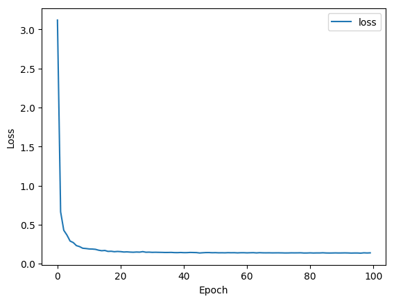
losses = rnn.train(X_train, Y_train, epochs=100)

With the increase in epochs, the loss gets smaller and smaller as the model learn:

Final Words & Resources

This was one of the most interesting concepts I have learned about ML and Deep Learning so far. So much complexity and things going on in a RNN model internally.

For more content on ML and my learning journey, take a look at the following resources:

• Machine Learning Research
• Recurrent Neural Networks cheatsheet
• NLP From Scratch: Translation with a Sequence to Sequence Network and Attention
• Deep Dive: Recurrent Neural Networks
• Building a Recurrent Neural Network From Scratch
• ML Learning Path

Twitter · Github