Building a Logistic Regression from Scratch with Python & Mathematics

2025-05-03

• 9 min read

Following the Linear Regression post, we are going to talk about Logistic Regression and classification problems, going from theory and mathematics to the implementation in Python.

Here is the table of contents:

Classification: classification problems and algorithms
Logistic regression for classification problems
Sigmoid function
Logistic regression probability output
Decision boundary and threshold
Loss and cost functions
Gradient Descent: model learning

Classification: problems and algorithms

A classification problem comes with predictors that are (un)correlated with an output.

The predictors are features of a dataset, and the output is a label or a class.

Examples of classification problems are

Classifying emails as “spam” or “not spam”
Classifying cancer tumors as “malignant” or “benign”

For binary classification problems, the output is described in pairs of 'positive'/'negative' such as 'yes'/'no, 'true'/'false' or '1'/'0'.

As learned before, linear regression is commonly used for continuous output that can range from negative infinity to positive infinity. Because it outputs a numerical value, it doesn't predict the probability of an example belonging to a particular class, which is required for a classification problem.

Linear regression also assumes a linear relationship between the independent variables (X) and the dependent variable (Y). In classification problems, the decision boundary between classes is often non-linear. Trying to fit a linear model to non-linearly separable data results in poor performance.

Logistic Regression

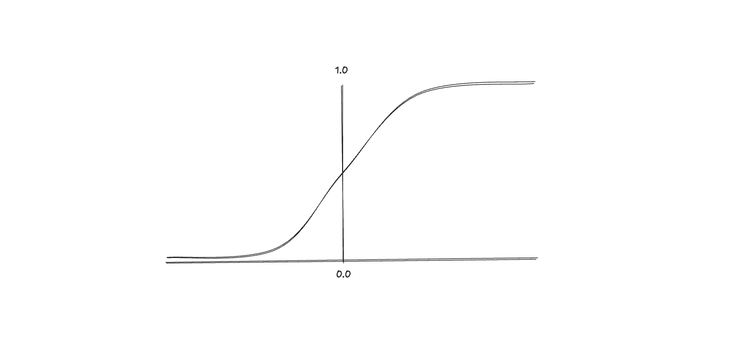
A binary classification prediction outputs 0 or 1, so we need a function that maps to these values. The sigmoid or logistic function can map all input values to values between 0 and 1.

The logistic function fits the data, and the algorithm outputs the threshold to separate the labels. The function is an S-shaped curve, as we can see below:

The sigmoid function follows this math equation:

g(z) = \frac{1}{1 + e^{-z}}

The implementation in Python is also quite simple:

def sigmoid(z):
    return 1 / (1 + np.exp(-z))

We use NumPy's exp function to calculate the exponential of values.

Similar to linear regression and neural networks, we compute the linear combination and then apply an activation function, in this case, the sigmoid function.

Linear combination:

f_{\mathbf{w},b}(\mathbf{x}^{(i)}) = \mathbf{w} \cdot \mathbf{x}^{(i)} + b

Activation function:

g(z)

where $z = f(x)$

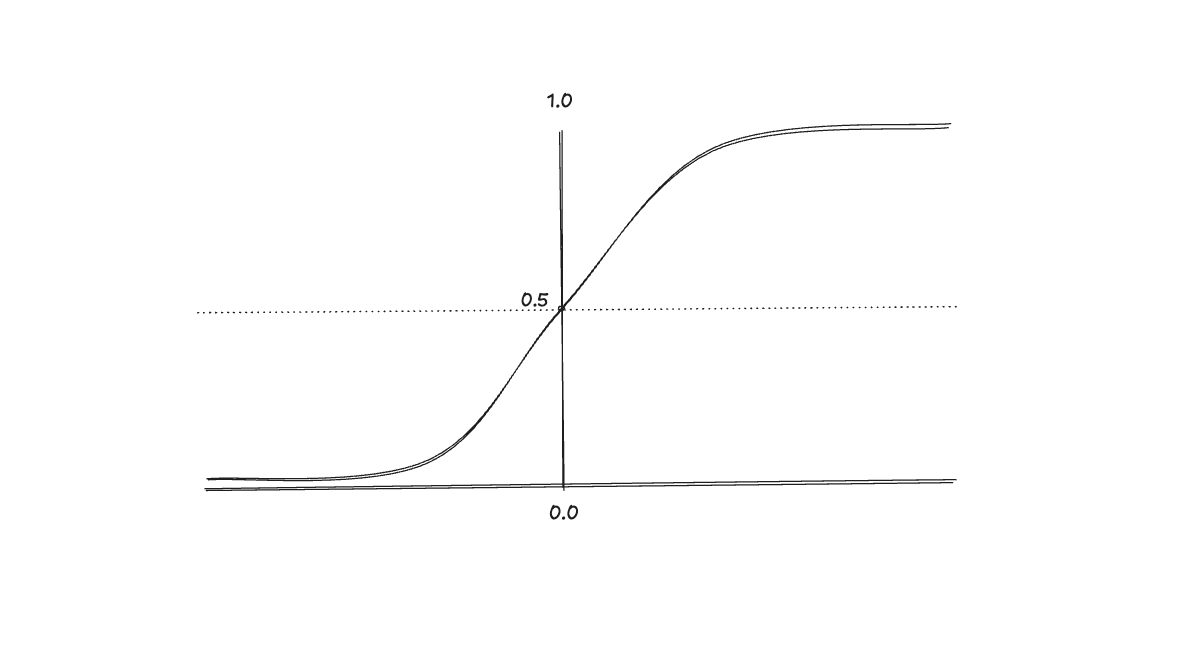
The logistic regression model will learn the decision boundary that will divide the feature space, and the algorithm can output the probability of $y = 1$ given $x$ .

A simple example is when the threshold is 0.5, so when $g(z) ≥ 0.5$ , $Y = 1$ , and $g(z) < 0.5$ , $Y = 0$ .

For a linear decision boundary, the function is a line that divides the feature space.

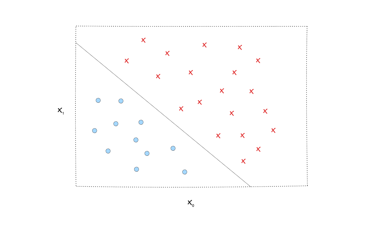
For complex problems where you can't split the labels with a line (linear decision boundary), we can come up with a more complex non-linear decision boundary to handle that.

Instead of using linear functions, we can use polynomial terms (circumference, ellipse, cluster/shape) so the decision boundary fits the data better.

Another important part of logistic regression is the output. For a binary classification, a logistic regression will output the probability of “label 1” and “label 2”.

For example, we have a dataset where we expect to predict if a cancer tumor is malignant (1) or benign (0). If the output for $Y = 1$ is 0.7, it means the model is predicting that there's a 70% chance of the tumor being malignant (1) and 30% benign.

Notice that summing up both probabilities, we have 1, or 100%.

Mathematically, this relationship is expressed as:

P(y=0 | x) = 1 - P(y=1 | x)

Therefore, if you sum the probabilities for both classes, you will indeed get 1 (or 100%):

P(y=0 | x) + P(y=1 | x) = (1 - P(y=1 | x)) + P(y=1 | x) = 1

Cost Function: measuring the error gap

Now, we have a first prediction using logistic regression. It computes a linear combination, applies an activation function called sigmoid or logistic function, and then outputs the probability of a class given the training data.

But calculating one prediction is not enough, and more often than not, it is misleading. What we want is to train the model with the dataset so it can learn. This learning process is basically computing the cost function and making the model update the parameters with the goal of minimizing the cost function.

The loss function is a measure of the difference between a single example output and its target value. The cost function is a measure of the losses over the whole training data.

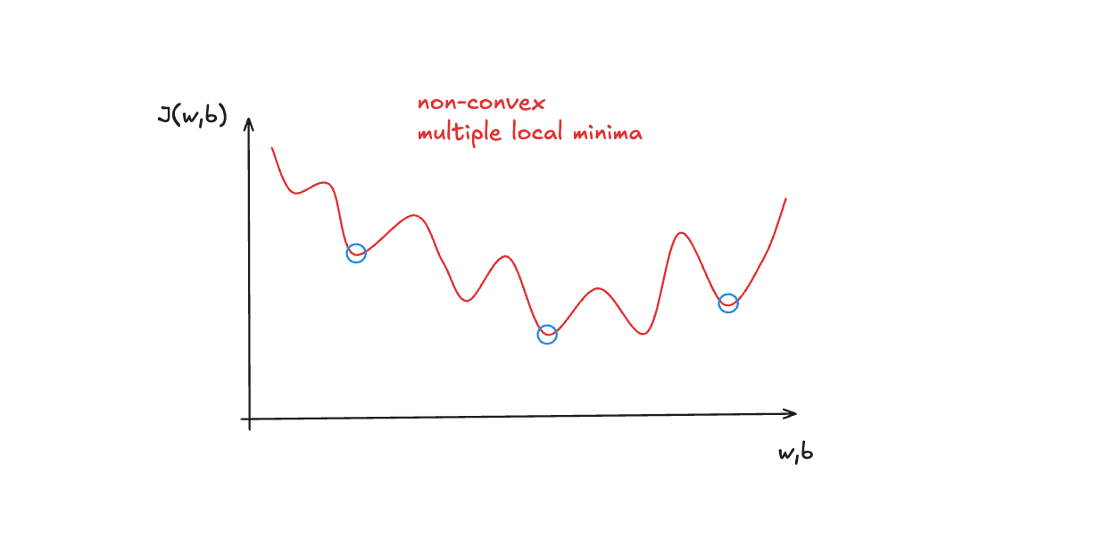
For linear regression, we used the squared error cost function, but it doesn't work well for logistic regression. It isn't as smooth as it is for linear regression. The non-linear nature of the model results in a non-convex cost function with many potential local minima.

For binary classification problems, we use a Log Loss, also called Binary Cross-Entropy. It fits better binary classification problems compared to the squared error function.

The equation for this loss function is defined:

$loss(f_{\mathbf{w},b}(\mathbf{x}^{(i)}), y^{(i)})$ is the cost for a single data point, which is:

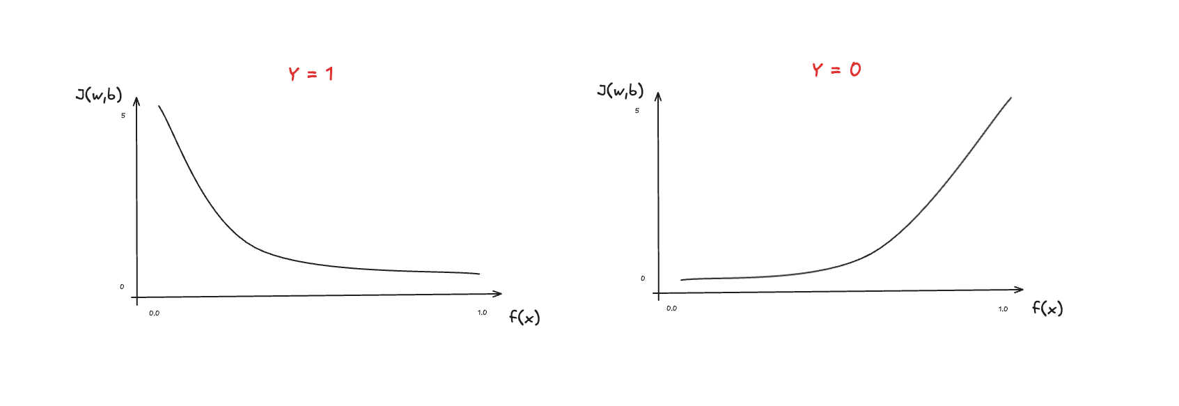
The idea of this loss function is to use two separate curves. One for the case when $Y = 1$ , and the other when $Y = 0$ .

The loss increases as the prediction differs from the target. Here is an illustration of the curves for when $Y = 1$ and $Y = 0$ :

The actual full equation for the loss function is defined:

loss(f_{\mathbf{w},b}(\mathbf{x}^{(i)}), y^{(i)}) = -y^{(i)} \log\left(f_{\mathbf{w},b}\left( \mathbf{x}^{(i)} \right) \right) - \left( 1 - y^{(i)}\right) \log \left( 1 - f_{\mathbf{w},b}\left( \mathbf{x}^{(i)} \right) \right)

At first, it can be a bit scary, but let's break it down and derive the equations we talked about before.

$f_{\mathbf{w},b}(\mathbf{x}^{(i)})$ is the model's prediction
$y^{(i)}$ is the target value.
$f_{\mathbf{w},b}(\mathbf{x}^{(i)}) = g(\mathbf{w} \cdot\mathbf{x}^{(i)}+b)$
$g$ is the sigmoid function.

When $y^{(i)} = 0$ , the left-hand term is eliminated:

When $y^{(i)} = 1$ , the right-hand term is eliminated:

Which falls into that previous equation:

This is how the loss function behaves. The cost function computes the loss of all $m$ training examples. It's the sum of the loss of all training examples over the number of training examples $m$ :

J(\mathbf{w},b) = \frac{1}{m} \sum_{i=0}^{m-1} \left[loss(f_{\mathbf{w},b}(\mathbf{x}^{(i)}), y^{(i)}) \right]

With the theory in mind, the implementation comes very simply. Here it is:

def compute_logistic_cost(X, y, w, b):
    m = X.shape[0]
    cost = 0.0

    for i in range(m):
        z_i = np.dot(X[i], w) + b
        f_wb_i = sigmoid(z_i)
        cost +=  -y[i] * np.log(f_wb_i) - (1 - y[i]) * np.log(1 - f_wb_i)

    cost = cost / m
    return cost

Here is the algorithm:

Loop through all the $m$ training examples
Compute the linear combination: $x * w + b$
Compute the sigmoid/logistic function
Compute the cost function: the sum of all losses over $m$ training examples. The average of losses

In previous posts, we talked about how to approach these algorithms with vectorization. So let's also transform it into a vectorized algorithm:

def compute_cost(X, y, w, b):
    m = X.shape[0]
    Z = np.dot(X, w) + b
    A = sigmoid(Z)
    cost = sum(-y * np.log(A) - (1 - y) * np.log(1 - A)) / m

    return cost

It's pretty much the same thing, but we compute everything in one go without the loop.

Gradient Descent: model learning

Gradient descent, as we learned before, is the algorithm to make the model “learn”, or in other words, update the parameters $W$ and $B$ based on the cost function.

The idea is to compute the gradient, a form of partial derivatives, for parameters $W$ and $B$ and update them.

The algorithm will update the parameters until convergence is reached.

The derivative of $J$ with respect to $W$ and $B$ looks like the following equation:

Here is the notation:

$m$ is the number of training examples in the dataset
$f_{\mathbf{w},b}(x^{(i)})$ is the model's prediction, while $y^{(i)}$ is the target
For a logistic regression model
- $z = \mathbf{w} \cdot \mathbf{x} + b$
- $f_{\mathbf{w},b}(x) = g(z)$ where $g(z)$ is the sigmoid function: $g(z) = \frac{1}{1+e^{-z}}$

The implementation is divided into two parts:

Compute the gradients
Gradient descent

The first function will calculate the gradient based on the cost, so it just needs to implement the code version of the following equation:

It receives $X$ , $y$ , and current $w$ and $b$ , and generates the gradients:

def compute_gradients(X, y, w, b):
    m, n = X.shape
    dj_dw = np.zeros((n,))
    dj_db = 0.

    for i in range(m):
        f_wb_i = sigmoid(np.dot(X[i], w) + b)
        err_i  = f_wb_i  - y[i]
        for j in range(n):
            dj_dw[j] = dj_dw[j] + err_i * X[i, j]
        dj_db = dj_db + err_i

    dj_dw = dj_dw / m
    dj_db = dj_db / m

    return dj_db, dj_dw

For each training example, we need to apply the sigmoid function and then compute the error to store the gradients for $w$ and $b$ .

The second part is the actual gradient descent algorithm, where it will use the gradients we computed earlier and update the parameters $w$ and $b$ until it finishes the number of iterations (hyperparameter) or until it reaches convergence.

Here is the implementation:

def gradient_descent(X, y, w_in, b_in, alpha, num_iters):
    J_history = []
    w = copy.deepcopy(w_in)
    b = b_in

    for i in range(num_iters):
        dj_db, dj_dw = compute_gradients(X, y, w, b)
        w = w - alpha * dj_dw
        b = b - alpha * dj_db
        J_history.append(compute_cost_logistic(X, y, w, b))

    return w, b, J_history

We just need to loop through the number of iterations passed to the model and keep updating the parameters $w$ and $b$ based on the computed gradients, and finish when the model reaches convergence.

After convergence, the model outputs the best, most optimized parameters. In other words, it learned through data the best parameter options to model and fit the data.

Final Words

This is one more step in my learning path studying ML/AI and biomedicine. This is the list of posts I've worked on:

In this article, I talk about this learning experience studying ML: My Experience Learning Machine Learning & Mathematics.

The next step is to write about decision trees, new neural network architectures (CNN, RNN), and more projects.

Resources

Hey! You may like this newsletter if you're enjoying this blog. ❤

✖

Twitter · Github