Self-Attention, Foundation Models, and the GPT Architecture from Scratch
Large language models like GPT, BERT, and Llama are built on top of the Transformer architecture. The core mechanism behind the Transformer architecture is called self-attention, which lets a model learn relationships between any two tokens in a sequence regardless of their distance.
In this post, I want to break down how this all works, from raw text to a working GPT-like model, building everything from scratch in Python and PyTorch.
My goal was to learn more about pretraining and finetuning to build foundation models. The main ideas come from the “Build a Large Language Model” book and the “Language Modeling from Scratch” course.
Here are the topics I'll cover:
- Tokenization
- Embeddings
- Simple Self-Attention
- Scaled Dot-Product Self-Attention with Trainable Weights
- Causal (Masked) Self-Attention
- Multi-Head Attention
- The Transformer Block
- The GPT Model Architecture
- Generating Text
- Pretraining
Tokenization and Embeddings
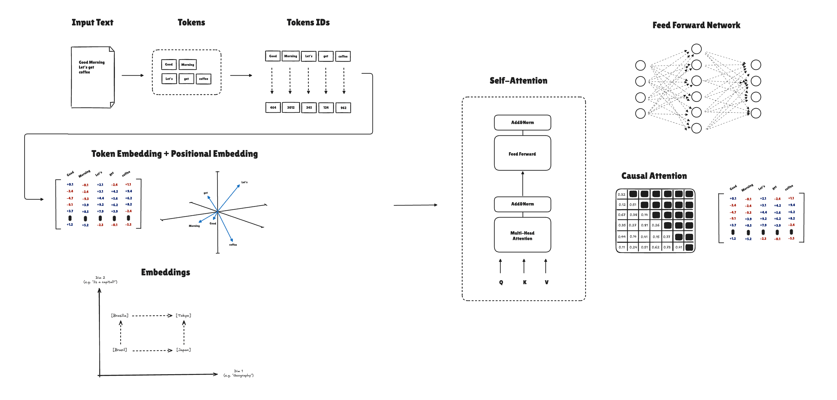
Before a language model can process text, we need to convert raw strings into numerical representations. The pipeline looks like this:
Input text → Tokens → Token IDs → Token Embeddings + Positional Embeddings → Input Embeddings
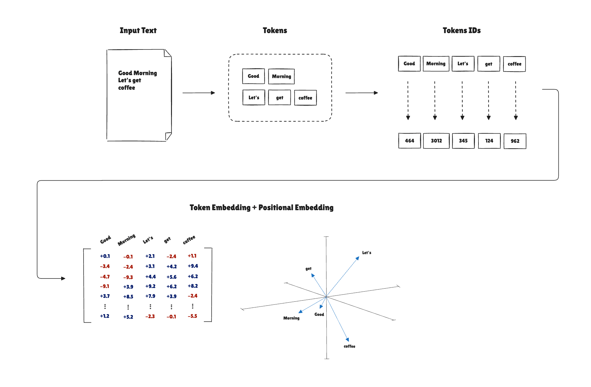
The first step is tokenization, the process of taking a string (a sequence of characters) and producing token IDs. Input text is split into tokens, and each token is converted to a token ID.
A simple, naive tokenizer splits text on punctuation and whitespace and maps each token to an integer ID. This process is called encoding:
import re

text = "Hello, world. Is this a test?"

# Split input text into tokens
tokens = re.split(r'([,.:;?_!"()\']|--|\s)', text)
tokens = [token for token in tokens if token.strip()]

# Transform tokens into token IDs
vocab = {token:integer for integer, token in enumerate(tokens)}
token_ids = [
  vocab[token] for token in tokens
]
The first step is just a text split based on special characters like punctuation and whitespace. The tokens look like this:
['Hello', ',', 'world', '.', 'Is', 'this', 'a', 'test', '?']
It's just a list of words.
Now we need to convert that into IDs. In a naive implementation, the IDs are created based on the generated tokens, and each token will be represented by an ID from 0 to the length of the tokens list. In this case, in the vocabulary, there will be 9 IDs (because we have 9 tokens).
Each token maps to the respective ID, generating the token IDs. These are the generated token IDs:
[0, 1, 2, 3, 4, 5, 6, 7, 8]
But now, if I add a good word to the input text, because we don't have this token in the vocabulary, the tokenizer will throw an error saying “the vocabulary doesn't have this token in the mapper”.
text = "Hello, world. Is this a good test?"
tokens = re.split(r'([,.:;?_!"()\']|--|\s)', text)
tokens = [token for token in tokens if token.strip()]
token_ids = [
  vocab[token] for token in tokens
]
# Traceback (most recent call last):
#   File "<stdin>", line 2, in <module>
# KeyError: 'good'
Generally, we have a bigger vocabulary with more tokens, so every input text can be handled by the tokenizer. But for this little experiment, let's use some special characters: <|unk|> for unknown tokens.
tokens.extend(["<|unk|>"])
vocab = {token:integer for integer, token in enumerate(tokens)}
token_ids = [
  vocab[token] if token in vocab
  else vocab["<|unk|>"] for token in tokens
]
We extend the tokens list with the <|unk|> token and add it to the vocabulary. When generating each token ID, unknown tokens in the vocabulary will be handled by the <|unk|> token.
This is the encoding process. The decode works backwards. We need to get the token IDs and transform them back to tokens, and then into the input text.
First, we start with the id_to_token mapper:
id_to_token = {v: k for k, v in vocab.items()}
And then, we can transform the token IDs back to tokens:
tokens = [
  id_to_token[token_id] if token_id in id_to_token
  else "<|unk|>" for token_id in token_ids
]
And finally, join the tokens into a string:
text = " ".join(tokens)
text = re.sub(r'\s+([,.:;?!"()\'])', r'\1', text)
text # 'Hello, world. Is this a good test? <|unk|>'
With the encoding and decoding explained, we can build a simple abstraction for the tokenizer. Let's call it SimpleTokenizer:
import re

class SimpleTokenizer:
  def __init__(self, vocab):
    self.token_to_id = vocab
    self.id_to_token = {v: k for k, v in vocab.items()}

  def encode(self, text):
    # Split input text into tokens (separate words)
    tokens = re.split(r'([,.:;?_!"()\']|--|\s)', text)
    tokens = [token for token in tokens if token.strip()]

    # Convert tokens to token IDs
    token_ids = [
      self.token_to_id[token] if token in self.token_to_id
      else self.token_to_id["<|unk|>"] for token in tokens
    ]

    return token_ids

  def decode(self, token_ids):
    # Convert token IDs to tokens
    tokens = [
      self.id_to_token[token_id] if token_id in self.id_to_token
      else "<|unk|>" for token_id in token_ids
    ]

    # Join tokens back into a string
    text = " ".join(tokens)
    text = re.sub(r'\s+([,.:;?!"()\'])', r'\1', text)
    return text
Let's test it:
text = "Hello, world. Is this a test?"
tokens = re.split(r'([,.:;?_!"()\']|--|\s)', text)
tokens = [token for token in tokens if token.strip()]
tokens.extend(["<|unk|>"])
vocab = {token:integer for integer, token in enumerate(tokens)}

tokenizer = SimpleTokenizer(vocab)
text = "Hello, world. Is this a good test?"
token_ids = tokenizer.encode(text) # [0, 1, 2, 3, 4, 5, 6, 9, 7, 8]
decoded_text = tokenizer.decode(token_ids) # Hello, world. Is this a <|unk|> test?
But this is a very naive implementation. The vocabulary is also too small. For the foundation model we will build, we need a better tokenizer.
For a more robust tokenizer, we'll use the tiktoken, a BPE tokenizer implemented by OpenAI.
import tiktoken

tokenizer = tiktoken.get_encoding("gpt2")

text = (
  "Good morning! I know a good place for coffee. Do you want to go? <|endoftext|> I see you there."
)

token_ids = tokenizer.encode(text, allowed_special={"<|endoftext|>"})
token_ids # [10248, 3329, 0, 314, 760, 257, 922, 1295, 329, 6891, 13, 2141, 345, 765, 284, 467, 30, 220, 50256, 314, 766, 345, 612, 13]

strings = tokenizer.decode(token_ids)
strings # Good morning! I know a good place for coffee. Do you want to go? <|endoftext|> I see you there.
The API looks pretty much the same way. We get a specific tokenizer (gpt2 in this case), and encode and decode the input text.
In the encoding process, it generates the token IDs and generates the string in the decoding task.
Embeddings
As stated in the previous section, token IDs are merely an arbitrary index. It has no inherent meaning. We need a better representation, that can be learned (through training), to give meaning and capture semantics.
This is when embeddings come into place. Technically, an embedding is a dense numerical vector. It's used as a representation of a word or a token in this context.
[2, 3, 5, 1] # word embedding 1
[2, 1, 5, 4] # word embedding 2
[2, 3, 8, 2] # word embedding 3
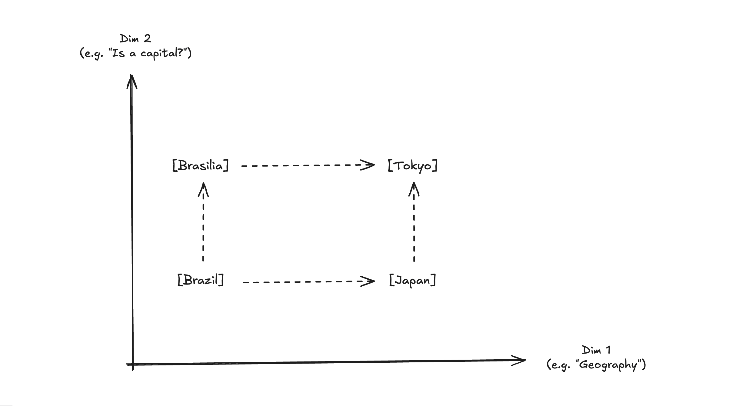
In a continuous vector space, two similar vectors (closeness, distance) are two similar words. In other words, they are semantically related because they are close in the vector space.
The direction of a vector tells us about the meaning, a relationship representation.
We need an embedding for each token in our “vocabulary,” so we should build a lookup table with token IDs as keys and embedding vectors as values. That way, every time we handle a token, we can use the lookup table to map it to the correct embedding.
When constructing this embedding lookup table, we need the intuition of what the “number of embeddings” and the “output dimension” mean.
Number of embeddings: the number of tokens in the vocabulary (token embedding), the number of positions (positional embedding). Each of them should have an embedding representation.Output dimension: the number of coordinates for a given item. It represents the traits, features, or characteristics of this item.
Let's see a simple example of using embeddings in PyTorch. Once we have the token IDs, we need to:
- Transform them into dense vectors through an embedding lookup table.
- This lookup table has shape
(vocab_size, embedding_dim), one row per token in the vocabulary.
import torch
import torch.nn as nn

input_ids = torch.tensor([2, 3, 5, 1])
vocab_size = 6
output_dim = 3

embedding_layer = nn.Embedding(vocab_size, output_dim)
embedding = embedding_layer(input_ids)
The embedding_layer is the lookup table and will be used to select the related embedding.
A lookup is just a matrix row selection. So, embedding_layer(input_ids) returns the rows at the given indices from the weight matrix. In other words, for a given token, it finds the related embedding vector.
We will see more of it in the training section, but the embeddings start as random vectors in the embedding space, and through training, the model learns to capture semantic meanings.
Another piece of intuition is how to adjust the output dimension to the vocabulary size. In summary, we need a large output dimension to encapsulate all possible characteristics of a large vocabulary.
- Few coordinates: small number of traits → underfitting
- Several coordinates: big number of traits → overfitting
The larger the vocabulary, the more characteristics are needed.
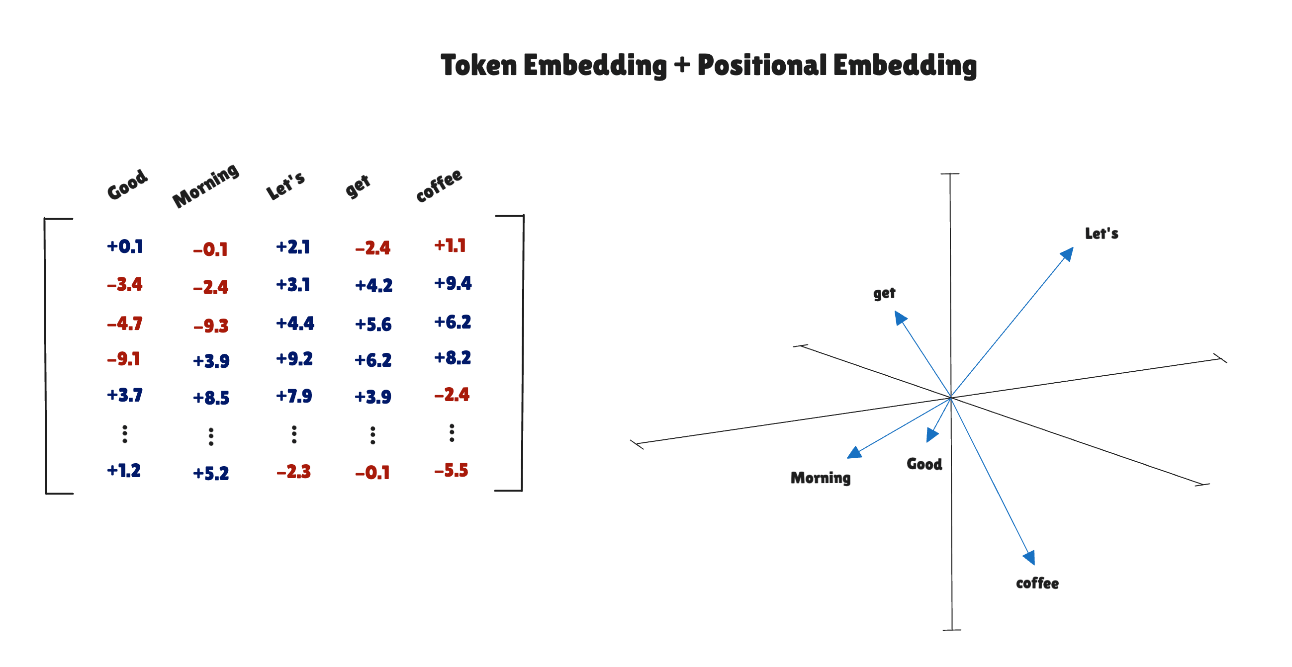
Token Embeddings
In the next two sections, we will talk about two parts of the embedding process of large language models: token and positional embeddings.
In token embeddings, we just build the embedding lookup table and map each token ID to an embedding vector, generating the token embedding.
Let's build the token IDs first:
import tiktoken
import torch
import torch.nn as nn

max_length = 4
text = "Good morning! I know a good place for coffee. Do you want to go? <|endoftext|> I see you there."

tokenizer = tiktoken.get_encoding("gpt2")
token_ids = tokenizer.encode(text, allowed_special={"<|endoftext|>"})
input = torch.tensor(token_ids[0:max_length])
Here is the breakdown:
- Our input is a simple one-sentence text.
- We use the GPT2 tokenizer
- We use only 4 tokens at a time (
max_length)
With that, we need our lookup table:
vocab_size = tokenizer.n_vocab # 50257
output_dim = 256
token_embedding_layer = nn.Embedding(vocab_size, output_dim)
Here, it is important to notice that, because we are using the GPT2 tokenizer, we are dealing with a 50257 vocabulary size. That means we need to compute an embedding table of 50257 rows. For the output dimension, we experiment with 256 characteristics.
That done, we can call it for our input:
token_embeddings = token_embedding_layer(input)
Positional Embeddings
The same token ID always maps to the same embedding vector, regardless of its position in the sequence. That means a pure token embedding has no concept of order. To handle this, we add a learned positional embedding to each token embedding.
Positional embeddings are exactly that. They give positional meaning to tokens in the sequence.
It follows a similar process: build an embedding table that encapsulates each position, and use it to map each position to an embedding vector.
Let's recap how the input looks like:
import tiktoken
import torch
import torch.nn as nn

max_length = 4
text = "Good morning! I know a good place for coffee. Do you want to go? <|endoftext|> I see you there."

tokenizer = tiktoken.get_encoding("gpt2")
token_ids = tokenizer.encode(text, allowed_special={"<|endoftext|>"})
input = torch.tensor(token_ids[0:max_length])
It's important to notice that the input holds 4 positions in this little experiment, and we will work with it for this positional embedding.
context_length = max_length
output_dim = 256
positional_embedding_layer = torch.nn.Embedding(context_length, output_dim)
And finally, we get the positional embedding, mapping each position to the embedding vector.
positions = torch.arange(context_length) # tensor([0, 1, 2, 3])
positional_embeddings = positional_embedding_layer(positions)
Input Embeddings
With the token and the positional embeddings in place, we can generate the input embeddings and use them in our foundation model.
input_embeddings = token_embeddings + positional_embeddings
The input embeddings are a simple addition of the token and positional embeddings.
Self-Attention
With the input embeddings in place, we can work on the self-attention layer, so the model can learn relationships between tokens. But before moving to the “learning” part, let's implement the building blocks to build this intuition on how self-attention works.
The pipeline looks like this:
inputs → dot products → attention scores → softmax → attention weights → weighted sum → context vectors
The whole idea here is to compute dot products between token pairs, normalize these attention scores with a softmax, and compute a weighted sum to generate context vectors.
From the previous section, we learned about token, positional, and input embeddings. Let's build a simple one to use for our attention mechanism.
max_length = 4
text = "Good morning! I know a good place for coffee. Do you want to go? <|endoftext|> I see you there."

tokenizer = tiktoken.get_encoding("gpt2")
token_ids = tokenizer.encode(text, allowed_special={"<|endoftext|>"})
inputs = torch.tensor(token_ids[0:max_length])

# === create token embeddings ===
vocab_size = tokenizer.n_vocab # 50257
output_dim = 3
token_embedding_layer = nn.Embedding(vocab_size, output_dim)
token_embeddings = token_embedding_layer(inputs)
# === // ===

# === create position embeddings ===
context_length = max_length
positional_embedding_layer = torch.nn.Embedding(context_length, output_dim)
positions = torch.arange(context_length)
positional_embeddings = positional_embedding_layer(positions)
# === // ===

# === create input embeddings ===
input_embeddings = token_embeddings + positional_embeddings
# === // ===
This outputs the input embeddings with shape (4, 3):
tensor([[ 0.9374,  3.6274, -0.1616],
        [-0.8188,  0.8241, -1.1497],
        [ 0.4806,  1.9741, -0.9867],
        [-1.1420, -0.0568, -0.3236]], grad_fn=<AddBackward0>)

# torch.Size([4, 3])
We will use this representation as the input embeddings for each token (Good, morning, !, I):
input_embeddings = torch.tensor(
  [[ 0.9374,  3.6274, -0.1616], # Good     (x^1)
   [-0.8188,  0.8241, -1.1497], # morning  (x^2)
   [ 0.4806,  1.9741, -0.9867], # !        (x^3)
   [-1.1420, -0.0568, -0.3236]] # I        (x^4)
) # shape: 4x3
To compute the attention scores, we need to compute the dot products between every pair of tokens. To make it more explicit, we can use torch.dot for every pair in the sequence with a for loop.
attn_scores = torch.empty(max_length, max_length)

for i, x_i in enumerate(input_embeddings):
    for j, x_j in enumerate(input_embeddings):
        attn_scores[i, j] = torch.dot(x_i, x_j)
This will produce a vector of shape (4, 4) (4x3 . 3x4 -> 4x4).
Using loops is not very performant. We'd better use matrix multiplication and compute all dot products simultaneously.
attn_scores = input_embeddings @ input_embeddings.T
This produces pretty much the same output as before in the loop.
The intuition behind it is that self-attention lets every token in a sequence "look at" every other token and decide how much to weight each one when building its own representation.
- Calculate how much the token should pay attention to all other tokens in the input sequence
- Learn the relationships and dependencies between tokens
Each row represents how much the token is paying attention to the other tokens (each column).
[[14.0628,  2.4075,  7.7707, -1.2242],
 [ 2.4075,  2.6712,  2.3675,  1.2603],
 [ 7.7707,  2.3675,  5.1015, -0.3417],
 [-1.2242,  1.2603, -0.3417,  1.4120]]

Attention scores for the string: "Good morning! I"
Tokens: ["Good", "morning", "!", "I"]
| Good | morning | ! | I | |
|---|---|---|---|---|
| Good | 14.0628 | 2.4075 | 7.7707 | -1.2242 |
| morning | 2.4075 | 2.6712 | 2.3675 | 1.2603 |
| ! | 7.7707 | 2.3675 | 5.1015 | -0.3417 |
| I | -1.2242 | 1.2603 | -0.3417 | 1.4120 |
Then, we apply softmax to produce attention weights. This is basically an attention score normalization, outputting a probability distribution, where each row is the probability distribution of how much the token is paying attention to the other tokens.
attn_weights = torch.softmax(attn_scores, dim=-1)
dim=-1 means softmax is applied row-wise, which makes sense in this context, because we want to know the probability distribution for each token (paired with the tokens in the sequence).
[[9.9814e-01, 8.6570e-06, 1.8475e-03, 2.2917e-07],
 [2.7931e-01, 3.6361e-01, 2.6838e-01, 8.8692e-02],
 [9.3101e-01, 4.1917e-03, 6.4523e-02, 2.7912e-04],
 [3.4046e-02, 4.0837e-01, 8.2288e-02, 4.7529e-01]]
| Good | morning | ! | I | |
|---|---|---|---|---|
| Good | 0.99814 | 0.0000087 | 0.0018475 | 0.0000002 |
| morning | 0.27931 | 0.36361 | 0.26838 | 0.088692 |
| ! | 0.93101 | 0.0041917 | 0.064523 | 0.0002791 |
| I | 0.034046 | 0.40837 | 0.082288 | 0.47529 |
Now we just need to generate the context vectors:
# 4x4 . 4x3 -> 4x3
context_vectors = attn_weights @ input_embeddings
After building attention weights, producing the relationship patterns between tokens, we compute the matrix multiplication of it with the input embeddings.
Now the context vectors came back to the initial shape of (4, 3).
It's a basic weighted average. Let's see an example:
context[morning] = 0.27931 · embed(Good)
                 + 0.36361 · embed(morning)
                 + 0.26838 · embed(!)
                 + 0.08869 · embed(I)
This translates to:
context[morning] = 0.27931 · [ 0.9374,  3.6274, -0.1616]  # Good     (x^1)
                 + 0.36361 · [-0.8188,  0.8241, -1.1497]  # morning  (x^2)
                 + 0.26838 · [ 0.4806,  1.9741, -0.9867]  # !        (x^3)
                 + 0.08869 · [-1.1420, -0.0568, -0.3236]  # I        (x^4)
Now, the input embeddings have contextual meaning, it gets from the attention mechanism.
In this first part, we build a simple self-attention implementation that uses only the input embeddings. No learnable parameters. This is what we are going to do now: add learnable parameters to the self-attention mechanism.
If you take each operation we've done and glue everything together, this is what we get at the end of it:
softmax(inputs @ inputs.T) @ inputs
If you look closely, this looks pretty similar to the Transformer's self-attention equation.
Instead of inputs, it uses . Rather than inputs, there is a . replaces inputs. And finally, there is an addition to the equation: squared d.
Let's break it down:
- : query vector
- : key vector
- : value vector
- : embedding dimension
To optimize the relationship and token patterns, we need learnable parameters. In practice, we are just attaching parameters (weight matrices) to the input embedding, producing the , , and vectors.
For large language models, we are talking about high dimensionality, not just 4 dimensions. That means the matrix multiplication when producing attention scores likely explodes (very large positive or negative numbers).
Large numbers break softmax because of exponentials. The fix is the square root of the dimension to stabilize the attention scores. The division by (where is the key dimension) prevents the dot products from growing too large as the embedding dimension increases, which would push softmax into regions with very small gradients.
Let's first start with the learnable parameters. We need to create the weight matrices for , , and vectors.
d_in = input_embeddings.shape[1]
d_out = 2

W_query = torch.nn.Parameter(torch.rand(d_in, d_out, requires_grad=False))
W_key   = torch.nn.Parameter(torch.rand(d_in, d_out, requires_grad=False))
W_value = torch.nn.Parameter(torch.rand(d_in, d_out, requires_grad=False))
d_in is the input dimension that should match the input embeddings dimension. And d_out is the dimension of the , , and vectors, which determines how rich the model representation is when computing attention. Larger d_out means richer and more expressive representations, but harder/more costly to train.
For learning purposes, we chose a small d_out and no optimization config (requires_grad=False) to understand how it works.
With the weight matrices in place, we attach them to the input embeddings, creating the , , and vectors.
Q = input_embeddings @ W_query
K = input_embeddings @ W_key
V = input_embeddings @ W_value
It is simply a matrix multiplication.
And then use them to compute attention scores, attention weights, and the context vectors, similar to what we've done before.
attention_scores = Q @ K.T
attention_weights = torch.softmax(attention_scores / K.shape[1] ** 0.5, dim=-1)
context_vectors = attention_weights @ V
In one pass, the equation code looks like this:
torch.softmax(Q @ K.T / K.shape[1] ** 0.5, dim=-1) @ V
The difference from the simple version: , , and now live in a learned subspace, so the model can express richer similarity patterns than raw dot products over input embeddings.
Causal (Masked) Self-Attention
Language models generate text left-to-right, one token at a time (an autoregressive system). When predicting token t, the model should not be able to see tokens at positions t+1, t+2, etc. — that would be leaking future information.
We enforce this by masking the upper triangle of the attention score matrix with before the softmax. After softmax, those entries become 0, so future tokens receive zero attention weight.
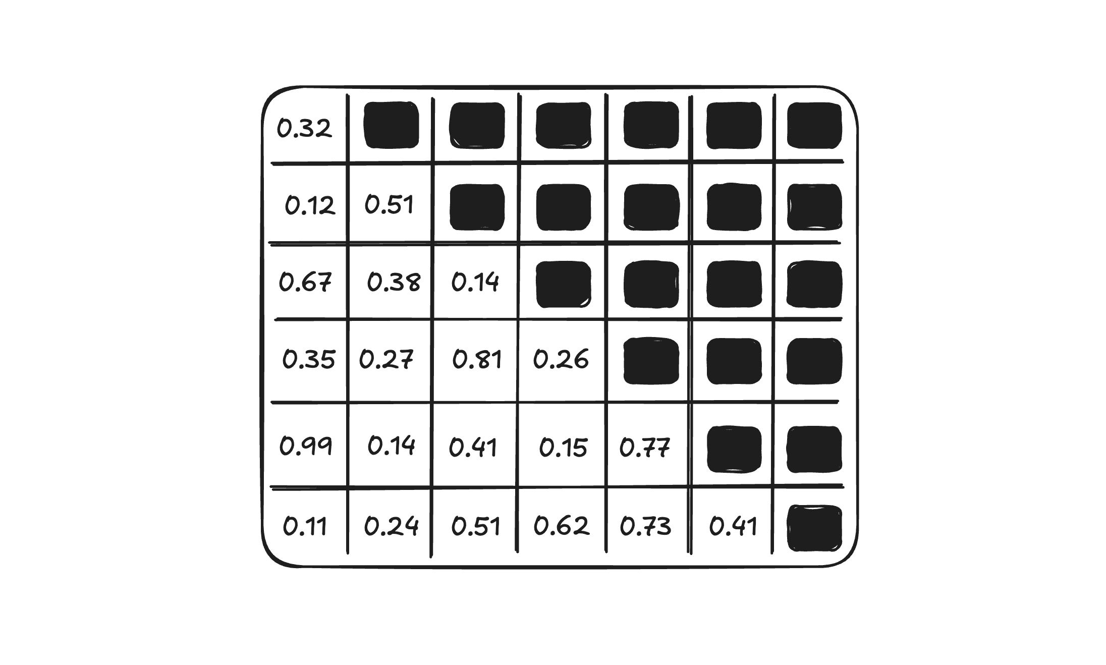
In terms of implementation, we can use the triu function from PyTorch to create this triangle mask and apply that to the attention scores:
mask = torch.triu(torch.ones(context_length, context_length), diagonal=1)
masked_attention_scores = attention_scores.masked_fill(mask.bool(), -torch.inf)
attention_weights = torch.softmax(masked_attention_scores / K.shape[1] ** 0.5, dim=-1)
context_vectors = attention_weights @ V
This is what it looks like when applying this mask to the attention scores:
# Attention Scores
[[16.5408, -2.5447,  8.5666, -6.8834],
 [-0.7491,  0.0398, -0.4083,  0.2480],
 [ 6.7302, -1.0641,  3.4779, -2.8250],
 [-2.9838,  0.4039, -1.5602,  1.1950]]

# Masked Attention Scores
[[16.5408,    -inf,    -inf,    -inf],
 [-0.7491,  0.0398,    -inf,    -inf],
 [ 6.7302, -1.0641,  3.4779,    -inf],
 [-2.9838,  0.4039, -1.5602,  1.1950]]

# Attention Weights
[[1.0000, 0.0000, 0.0000, 0.0000],
 [0.3640, 0.6360, 0.0000, 0.0000],
 [0.9055, 0.0037, 0.0908, 0.0000],
 [0.0295, 0.3236, 0.0807, 0.5662]]
We can see the mask affecting the attention scores by filling the -inf values into the upper triangle of the matrix, and then, when applying softmax, it normalizes it to 0.
Dropout
We also apply dropout to the attention weights after the softmax. This randomly zeros some entries during training, acting as regularization and preventing the model from over-relying on specific tokens.
Let's see a simple example first:
dropout = torch.nn.Dropout(0.5)
example = torch.ones(6, 6)
#  tensor([[1., 1., 1., 1., 1., 1.],
#         [1., 1., 1., 1., 1., 1.],
#         [1., 1., 1., 1., 1., 1.],
#         [1., 1., 1., 1., 1., 1.],
#         [1., 1., 1., 1., 1., 1.],
#         [1., 1., 1., 1., 1., 1.]])

dropout(example)
#  tensor([[2., 2., 0., 2., 2., 2.],
#         [2., 2., 2., 2., 0., 2.],
#         [0., 0., 0., 2., 2., 0.],
#         [2., 2., 2., 0., 0., 0.],
#         [0., 2., 2., 2., 0., 2.],
#         [2., 2., 2., 0., 2., 2.]])
Using the Dropout, it randomly sets some of the entries to zero.
Now, we apply that to the attention weights, after the softmax.
mask = torch.triu(torch.ones(context_length, context_length), diagonal=1)
masked_attention_scores = attention_scores.masked_fill(mask.bool(), -torch.inf)
attention_weights = torch.softmax(masked_attention_scores / K.shape[1] ** 0.5, dim=-1)
dropout = torch.nn.Dropout(0.5)
attention_weights = dropout(attention_weights)
context_vectors = attention_weights @ V
In this example, we set 50% of the entries to zero.
To complete this part, let's put everything together in a SelfAttention class so we can reuse that abstraction as much as we want.
Here's the full SelfAttention module:
class SelfAttention(nn.Module):
  def __init__(self, d_in, d_out, dropout, qkv_bias=False):
    super().__init__()
    self.W_query = nn.Linear(d_in, d_out, bias=qkv_bias)
    self.W_key = nn.Linear(d_in, d_out, bias=qkv_bias)
    self.W_value = nn.Linear(d_in, d_out, bias=qkv_bias)
    self.dropout = nn.Dropout(dropout)

  def forward(self, x):
    Q = self.W_query(x)
    K = self.W_key(x)
    V = self.W_value(x)

    attention_scores = Q @ K.T
    context_length = attention_scores.shape[0]
    mask = torch.triu(torch.ones(context_length, context_length), diagonal=1)
    masked_attention_scores = attention_scores.masked_fill(mask.bool(), -torch.inf)
    attention_weights = torch.softmax(masked_attention_scores / K.shape[1] ** 0.5, dim=-1)
    attention_weights = self.dropout(attention_weights)
    context_vectors = attention_weights @ V
    return context_vectors
Let's see it in action.
Create the input embedding first:
max_length = 6
text = "Good morning! I know a good place for coffee. Do you want to go? <|endoftext|> I see you there."

tokenizer = tiktoken.get_encoding("gpt2")
token_ids = tokenizer.encode(text, allowed_special={"<|endoftext|>"})
inputs = torch.tensor(token_ids[0:max_length])

# === create token embeddings ===
vocab_size = tokenizer.n_vocab # 50257
output_dim = 3
token_embedding_layer = nn.Embedding(vocab_size, output_dim)
token_embeddings = token_embedding_layer(inputs)
# === // ===

# === create position embeddings ===
context_length = max_length
positional_embedding_layer = torch.nn.Embedding(context_length, output_dim)
positions = torch.arange(context_length)
positional_embeddings = positional_embedding_layer(positions)
# === // ===

# === create input embeddings ===
input_embeddings = token_embeddings + positional_embeddings
# === // ===
And now, use it on the SelfAttention:
d_in = input_embeddings.shape[1]
d_out = 2

self_attention = SelfAttention(d_in, d_out, dropout=0.5)
self_attention(input_embeddings)
That is the printed version of each step. We can see the mask being applied correctly, softmax normalizing the scores, dropout zeroing some values, and outputting the context vectors.
# Attention scores:
#  tensor([[ 2.7144e-02,  6.1322e-02, -1.1982e-01, -2.0707e-01, -7.9423e-02, -7.8579e-02],
#         [-8.9638e-02,  6.5061e-01,  1.8978e-01,  6.0494e-02, -1.9703e-01, -1.8121e-01],
#         [-8.6843e-02,  7.3455e-01,  1.5870e-01, -1.7545e-02, -2.4700e-01, -2.2940e-01],
#         [-9.9800e-02,  1.4635e-01,  3.5080e-01,  4.8966e-01,  9.1835e-02, 9.6841e-02],
#         [-4.7818e-04,  3.0528e-01, -7.1828e-02, -2.2018e-01, -1.6354e-01, -1.5687e-01],
#         [-1.4737e-03, -1.5567e-01,  4.3272e-02,  1.2254e-01,  8.6330e-02, 8.2962e-02]], grad_fn=<MmBackward0>)
#
# Masked attention scores:
#  tensor([[ 2.7144e-02, -inf, -inf, -inf, -inf, -inf],
#         [-8.9638e-02,  6.5061e-01, -inf, -inf, -inf, -inf],
#         [-8.6843e-02,  7.3455e-01,  1.5870e-01, -inf, -inf, -inf],
#         [-9.9800e-02,  1.4635e-01,  3.5080e-01,  4.8966e-01, -inf, -inf],
#         [-4.7818e-04,  3.0528e-01, -7.1828e-02, -2.2018e-01, -1.6354e-01, -inf],
#         [-1.4737e-03, -1.5567e-01,  4.3272e-02,  1.2254e-01,  8.6330e-02, 8.2962e-02]], grad_fn=<MaskedFillBackward0>)
#
# Attention weights:
#  tensor([[1.0000, 0.0000, 0.0000, 0.0000, 0.0000, 0.0000],
#         [0.3721, 0.6279, 0.0000, 0.0000, 0.0000, 0.0000],
#         [0.2514, 0.4494, 0.2991, 0.0000, 0.0000, 0.0000],
#         [0.1968, 0.2342, 0.2706, 0.2985, 0.0000, 0.0000],
#         [0.2025, 0.2513, 0.1925, 0.1733, 0.1804, 0.0000],
#         [0.1627, 0.1459, 0.1679, 0.1776, 0.1731, 0.1727]],
#        grad_fn=<SoftmaxBackward0>)
#
# Dropout attention weights:
#  tensor([[0.0000, 0.0000, 0.0000, 0.0000, 0.0000, 0.0000],
#         [0.0000, 0.0000, 0.0000, 0.0000, 0.0000, 0.0000],
#         [0.5029, 0.0000, 0.5982, 0.0000, 0.0000, 0.0000],
#         [0.0000, 0.0000, 0.5412, 0.0000, 0.0000, 0.0000],
#         [0.4049, 0.5026, 0.3850, 0.3466, 0.0000, 0.0000],
#         [0.3254, 0.2918, 0.3359, 0.3552, 0.0000, 0.3454]],
#        grad_fn=<MulBackward0>)
#
# Context vectors:
#  tensor([[0.0000, 0.0000],
#         [0.0000, 0.0000],
#         [0.7736, 0.6035],
#         [0.7981, 0.3194],
#         [1.3495, 0.1422],
#         [1.2322, 0.0119]], grad_fn=<MmBackward0>)
Multi-Head Attention
A single attention head looks at the sequence through one "lens". Multi-head attention runs several attention heads in parallel, each with its own , , , and then concatenates the results. This allows the model to jointly attend to information from different representation subspaces.
The idea of a simple multi-head attention implementation is to compute attention-based context vectors for each “head” and then concatenate them together to produce the final context vectors output.
To do this, we need to loop N times (the number of heads) to produce the context vector for each head.
nn.ModuleList([
  SelfAttention(d_in, d_out, dropout, qkv_bias)
  for _ in range(num_heads)
])

context_vectors = [head(x) for head in self.heads]
And then, concatenate them.
torch.cat(context_vectors, dim=-1)
Moving it to a class-based abstraction, here is the whole implementation:
class MultiHeadAttentionStack(nn.Module):
  def __init__(self, d_in, d_out, dropout, num_heads, qkv_bias=False):
    super().__init__()
    self.num_heads = num_heads
    self.heads = nn.ModuleList([
      SelfAttention(d_in, d_out, dropout, qkv_bias)
      for _ in range(num_heads)
    ])

  def forward(self, x):
    return torch.cat([head(x) for head in self.heads], dim=-1)
Using our input_embeddings created previously, let's test the multi-head attention.
d_in = input_embeddings.shape[1]
d_out = 2

multi_head_attention = MultiHeadAttentionStack(d_in=d_in, d_out=d_out, dropout=0.5, num_heads=2)
context_vectors = multi_head_attention(input_embeddings)

#  tensor([[ 0.0000,  0.0000,  0.0000,  0.0000],
#          [ 0.7251,  0.2976,  0.8039,  0.9723],
#          [ 0.0000,  0.0000,  1.5051,  0.3576],
#          [ 0.8013, -0.2476,  0.3532, -3.3635],
#          [ 0.6733,  0.7412,  0.5880,  0.1965],
#          [ 0.5311, -0.1694, -0.0895, -1.9240]], grad_fn=<CatBackward0>)
With one head, we produced a vector of shape (6, 2). With 2 heads, because we concatenate the context vectors of each head together, we produce a vector of shape (6, 4).
One question comes to mind when we see this: why not increase the output dimension from 2 to 4 using only one head? How's that different than using 2 heads? Won't this produce the same output?
The answer lies in how the attention is computed. With one head, increasing the output dimension from 2 to 4 improves how the model learns the input representation, but all 4 output dimensions use the same attention weights.
The single head must commit to one way of "looking" at the context, and every dimension of the output is a weighted sum with that same distribution.
With 2 heads (multi-head attention), attention weights are computed independently for each head, meaning they produce different outputs using two independent attention weight vectors.
Each head can specialize in capturing a different relational structure in the input, producing richer representations.
An example of capturing different representations would be a language model with heads, one capturing synthetic, another positional, another focused on semantics, etc.
The Transformer Block
To build a transformer block, we took the first step, which was the multi-head attention. Look at how the transformer block works:
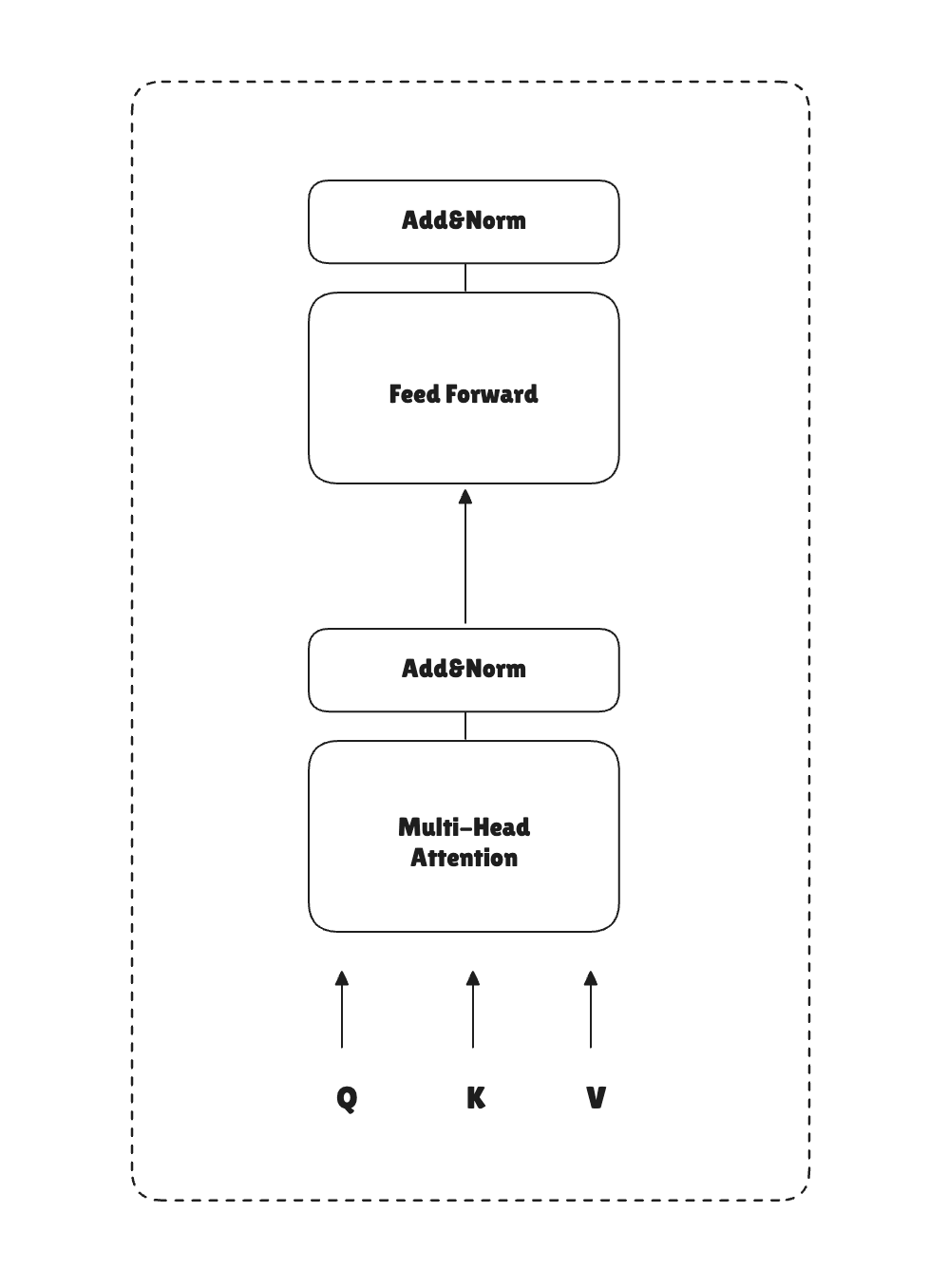
The Transformer block wraps multi-head attention with two additional components: a feed-forward network (FFN) and residual connections with layer normalization. Both are essential for training deep networks.
Let's build these two blocks, and then encapsulate everything into the transformer block.
Starting with the feed-forward network, here is the implementation:
class FeedForward(nn.Module):
    def __init__(self, cfg):
        super().__init__()
        self.layers = nn.Sequential(
            nn.Linear(cfg["emb_dim"], 4 * cfg["emb_dim"]),
            nn.GELU(),
            nn.Linear(4 * cfg["emb_dim"], cfg["emb_dim"]),
        )

    def forward(self, x):
        return self.layers(x)
It's a 2-layer MLP applied to each input token:
- Expand: a linear layer projects each token's embedding from
emb_dim→4 × emb_dim, making the representation 4× wider - Activate: GELU introduces non-linearity, allowing the network to learn non-linear functions
- Contract: a second linear layer projects back from
4 × emb_dim→emb_dim, restoring the original dimension
The next step is to implement the layer normalization.
This layer normalizes each token's embedding vector to have zero mean and unit variance, then applies learned scale and shift parameters.
class LayerNorm(nn.Module):
    def __init__(self, embedding_dim, eps=1e-5):
        super().__init__()
        self.eps = eps
        self.scale = nn.Parameter(torch.ones(embedding_dim))
        self.shift = nn.Parameter(torch.zeros(embedding_dim))

    def forward(self, x):
        mean = x.mean(dim=-1, keepdim=True)
        var = x.var(dim=-1, keepdim=True, unbiased=False)
        normalized_x = (x - mean) / torch.sqrt(var + self.eps)
        return self.scale * normalized_x + self.shift
As activations flow through many transformer blocks, their scales can drift (grow very large or shrink). The idea is that the layer normalization keeps the token's representation stable throughout the whole network.
With the feed-forward network and the layer normalization block implemented, we can encapsulate everything into the transformer block.
class TransformerBlock(nn.Module):
    def __init__(self, cfg):
        super().__init__()
        self.attention = MultiHeadAttention(
            d_in=cfg["emb_dim"],
            d_out=cfg["emb_dim"],
            context_length=cfg["context_length"],
            num_heads=cfg["n_heads"],
            dropout=cfg["drop_rate"],
            qkv_bias=cfg["qkv_bias"]
        )
        self.ff = FeedForward(cfg)
        self.layer_norm1 = LayerNorm(cfg["emb_dim"])
        self.layer_norm2 = LayerNorm(cfg["emb_dim"])
        self.dropout = nn.Dropout(cfg["drop_rate"])

    def forward(self, x):
        shortcut = x
        x = self.layer_norm1(x)
        x = self.attention(x)
        x = self.dropout(x)
        x = x + shortcut

        shortcut = x
        x = self.layer_norm2(x)
        x = self.ff(x)
        x = self.dropout(x)
        x = x + shortcut
        return x
Residual connections add the block's input back to its output (x = x + f(x)). This preserves gradient flow through very deep networks and lets each block learn an incremental refinement rather than a full transformation.
The full Transformer block applies layer norm before each sub-layer (pre-norm):
- Layer normalization
- Attention block
- Dropout
- Residual connection
We do this two times and return the output.
The GPT Model Architecture
Stacking multiple Transformer blocks on top of token and positional embeddings + an output head gives us a GPT-like decoder model.
class GPTModel(nn.Module):
    def __init__(self, cfg):
        super().__init__()
        self.token_embedding = nn.Embedding(cfg["vocab_size"], cfg["emb_dim"])
        self.positional_embedding = nn.Embedding(cfg["context_length"], cfg["emb_dim"])
        self.dropout_embedding = nn.Dropout(cfg["drop_rate"])
        self.transformer_blocks = nn.Sequential(
            *[TransformerBlock(cfg)
              for _ in range(cfg["n_layers"])]
        )
        self.final_norm = LayerNorm(cfg["emb_dim"])
        self.out_head = nn.Linear(cfg["emb_dim"], cfg["vocab_size"], bias=False)

    def forward(self, token_ids):
        _, seq_len = token_ids.shape
        token_embeddings = self.token_embedding(token_ids)
        positional_embedddings = self.positional_embedding(torch.arange(seq_len, device=token_ids.device))
        x = token_embeddings + positional_embedddings
        x = self.dropout_embedding(x)
        x = self.transformer_blocks(x)
        x = self.final_norm(x)
        logits = self.out_head(x)
        return logits
We have three different dropouts here:
- Embedding dropout: Prevents the model from over-relying on specific positions
- Post-attention dropout: Regularizes the information gathered from other tokens
- Post-feedforward dropout: Regularizes the per-token computation
The output is a tensor of logits with shape (batch_size, seq_len, vocab_size) — one score per vocabulary token, for each position. No softmax is applied inside the model; that happens in the loss function during training or in the sampling step during inference.
Generating Text
Now that we have our very rudimentary GPT model, let's use it to generate some text for us.
We'll use this generate_text function to help us with predicting the next token and generating the sentence based on the input passed:
def generate_text(model, idx, max_new_tokens, context_size, temperature=1.0, top_k=None):
    for _ in range(max_new_tokens):
        idx_cond = idx[:, -context_size:]
        with torch.no_grad():
            logits = model(idx_cond)

        logits = logits[:, -1, :]

        if top_k is not None:
            top_k_logits, _ = torch.topk(logits, top_k)
            logits = torch.where(
                logits < top_k_logits[:, -1],
                -float('inf'),
                logits
            )

        if temperature > 0.0:
            logits = logits / temperature
            probas = torch.softmax(logits, dim=-1)
            idx_next = torch.multinomial(probas, num_samples=1)
        else:
            probas = torch.softmax(logits, dim=-1)
            idx_next = torch.argmax(probas, dim=-1, keepdim=True)

        idx = torch.cat((idx, idx_next), dim=1)

    return idx
At inference time, we feed the model a sequence of token IDs and iteratively sample the next token. The key choices are temperature (which controls randomness) and top-k (which restricts sampling to the most likely tokens).
Temperature divides the logits before softmax:
T < 1— amplifies the gap between logits, making the model more deterministic and repetitiveT = 1— no change from the model's natural distributionT > 1— flattens the distribution, producing more varied (and potentially incoherent) output
Top-k sampling zeroes out all but the top-k logits (by setting them to ) before applying softmax, preventing the model from sampling very unlikely tokens.
Running this on an untrained model with top_k=25 and temperature=1.4 will produce random tokens — training is the step that teaches the model to generate coherent text.
The GPT-2 124M configuration looks like this:
GPT_CONFIG_124M = {
    "vocab_size": 50257,
    "context_length": 256,
    "emb_dim": 768,
    "n_heads": 12,
    "n_layers": 12,
    "drop_rate": 0.1,
    "qkv_bias": False
}
With 12 transformer blocks, 12 attention heads, and 768-dimensional embeddings, this model has approximately 124 million parameters.
Let's create an instance of our model:
model = GPTModel(GPT_CONFIG_124M)
model.eval()
And call the helper function to generate the text for us:
tokenizer = tiktoken.get_encoding("gpt2")

token_ids = generate_text(
    model=model,
    token_ids=text_to_token_ids("Good morning!", tokenizer),
    max_new_tokens=15,
    context_size=GPT_CONFIG_124M["context_length"],
    top_k=25,
    temperature=1.4
)

# Token IDs:
# tensor([[10248,  3329,     0, 31099, 47043, 35018, 25097, 29356, 16620, 33263,
#          38319, 36129, 44830,  9176, 31307, 41526,  6557, 15759]])
We can use the token_ids_to_text to decode these IDs back into the words:
token_ids_to_text(token_ids, tokenizer)
# Good morning! commute Chinatown intervenedMovieloadertalkuku dissectaqu Sind roles resilience TOMáavior
This produces a very weird sentence. One, because it's just generating text, it's not trained/finetuned, and two, because it's using a high top_k and temperature.
Pretraining
Getting the same idea from the “Build a Large Language Model (From Scratch)” book, we will be using Edith Wharton's short story The Verdict as the dataset for the model training.
This section is called pretraining, where we are going to do 3 things:
- Create datasets + dataloaders
- Define our loss function
- Train the language model
Before a language model can learn anything, the raw text must be transformed into a structured, numerical format that PyTorch can consume during training. We will be working on the construction of a custom Dataset class and a DataLoader pipeline.
Sliding Window Chunking
Language models are trained on fixed-length sequences. Since "The Verdict" is a continuous stream of ~5,000 tokens, it must be divided into overlapping chunks of length max_length. This is done with a sliding window:
for i in range(0, len(token_ids) - max_length, stride):
    input_chunk  = token_ids[i : i + max_length]
    target_chunk = token_ids[i + 1 : i + max_length + 1]
Two parameters handle this process:
max_length: the number of tokens in each input sequence, equal to the model'scontext_length(256 tokens in this configuration). This sets the maximum span of context the model can attend to during a single forward pass.stride— the step size between consecutive windows. Whenstride == max_length, windows are non-overlapping, and each token appears in exactly one training sample. Whenstride < max_length, windows overlap, and tokens appear in multiple samples, which can improve gradient signal density but also increase training time and the risk of overfitting.
The target sequence is simply the input sequence shifted one position to the right. This implements next-token prediction: for every position (t) in the input, the model is trained to predict the token at position (t+1). This is also called a self-supervised learning that requires no labeled data (the labels are derived from the input itself).
The GPTDataset Class
With that, let's build our class abstraction to encapsulate this logic:
class GPTDataset(Dataset):
    def __init__(self, text, tokenizer, max_length, stride):
        self.input_ids = []
        self.target_ids = []
        token_ids = tokenizer.encode(text)
        for i in range(0, len(token_ids) - max_length, stride):
            input_chunk  = token_ids[i : i + max_length]
            target_chunk = token_ids[i + 1 : i + max_length + 1]
            self.input_ids.append(torch.tensor(input_chunk))
            self.target_ids.append(torch.tensor(target_chunk))

    def __len__(self):
        return len(self.input_ids)

    def __getitem__(self, idx):
        return self.input_ids[idx], self.target_ids[idx]
GPTDataset implements 3 methods:
__len__: returns the total number of samples.__getitem__: returns a single(input_ids, target_ids)pair as a tuple of tensors.__init__: creates the input and target chunks
The create_dataloader
The create_dataloader creates the dataloader with the dataset:
def create_dataloader(text, batch_size=4, max_length=256, stride=128, shuffle=True, drop_last=True, num_workers=0):
  tokenizer = tiktoken.get_encoding("gpt2")
  dataset = GPTDataset(text, tokenizer, max_length, stride)
  dataloader = DataLoader(
    dataset,
    batch_size=batch_size,
    shuffle=shuffle,
    drop_last=drop_last,
    num_workers=num_workers
  )

  return dataloader
The dataloader handles batching, shuffling, and parallel loading.
Train/Validation Split
train_ratio  = 0.90
split_index  = int(train_ratio * len(raw_text))
train_data   = raw_text[:split_index]
val_data     = raw_text[split_index:]
The raw text is split at the character level (before tokenization) into a 90% training set and 10% validation set. The split is positional, not random. The first 90% of the story becomes training data, and the remaining 10% becomes the validation set.
This chronological split is appropriate for a single continuous document: splitting randomly at the character level would slice through sentences, creating nonsensical fragments at the boundaries. A positional split ensures both partitions contain grammatically complete, contextually coherent text.
With a story of roughly 36,000 characters, the validation set contains approximately 3,600 characters. After tokenization, this yields around 750–900 tokens — just a few full-length sequences at context_length=256.
Putting It Together
The two dataloaders are constructed using the same create_dataloader factory but with configurations tuned to their respective roles:
train_dataloader = create_dataloader(
  train_data,
  batch_size=2,
  max_length=GPT_CONFIG_124M["context_length"],
  stride=GPT_CONFIG_124M["context_length"],
  drop_last=True,
  shuffle=True,
  num_workers=0
)

val_dataloader = create_dataloader(
  val_data,
  batch_size=2,
  max_length=GPT_CONFIG_124M["context_length"],
  stride=GPT_CONFIG_124M["context_length"],
  drop_last=False,
  shuffle=False,
  num_workers=0
)
These two dataloaders are passed directly into the training loop, where the model iterates over train_dataloader to update weights and periodically evaluate on val_dataloader to monitor generalization.
Training
The first step in the training process is to choose the loss function that fits the problem at hand well. Next-token prediction is fundamentally a multi-class classification problem. It should choose one token over N possible tokens (one output, many possible classes).
Cross-entropy is a good choice for this problem. It measures how well the predicted probability distribution over the vocabulary matches the true next token. And it penalizes the model when it assigns low probability to the correct token.
def calculate_loss_batch(input_batch, target_batch, model):
  logits = model(input_batch)
  loss = torch.nn.functional.cross_entropy(logits.flatten(0, 1), target_batch.flatten())
  return loss
In the training process, we will also need to evaluate the model, basically, by calculating the average loss across all batches in a dataloader.
def calculate_loss_loader(data_loader, model):
  total_loss = 0.

  for (input_batch, target_batch) in data_loader:
    loss = calculate_loss_batch(input_batch, target_batch, model)
    total_loss += loss.item()

  return total_loss / len(data_loader)
It accumulates the losses of every batch to compute the mean. This gives a single number representing how well the model is doing over the entire dataset.
We need this for both the training and the validation sets.
def evaluate_model(model, train_loader, val_loader):
    model.eval()

    with torch.no_grad():
        train_loss = calculate_loss_loader(train_loader, model)
        val_loss = calculate_loss_loader(val_loader, model)

    model.train()
    return train_loss, val_loss
evaluate_model should receive the train and validation loader to compute this single-value loss. This will help us keep track of the losses across the training process. It's purely diagnostic.
The training process is the standard approach for training deep learning models.
train_losses, val_losses, track_tokens_seen = [], [], []
tokens_seen, global_step = 0, -1

for epoch in range(num_epochs):
    model.train()
    for input_batch, target_batch in train_loader:
        optimizer.zero_grad()
        loss = calculate_loss_batch(input_batch, target_batch, model)
        loss.backward()
        optimizer.step()
        tokens_seen += input_batch.numel()
        global_step += 1
Training runs for multiple epochs, iterating over batches each time. This standard approach covers model prediction (logits), loss computation, backpropagation, and parameter updates.
For diagnostics, we run this evaluation to keep track of the losses in the loop:
if global_step % eval_freq == 0:
      train_loss, val_loss = evaluate_model(model, train_loader, val_loader)
      train_losses.append(train_loss)
      val_losses.append(val_loss)
      track_tokens_seen.append(tokens_seen)
      print(f"Ep {epoch+1} (Step {global_step:06d}): "
            f"Train loss {train_loss:.3f}, "
            f"Val loss {val_loss:.3f}"
      )
To finish this training function, we add a (qualitative) sanity test, so we can check what the model is producing and pair it with the loss in each step.
def generate_and_print_sample(model, tokenizer, start_context):
    model.eval()
    context_size = model.positional_embedding.weight.shape[0]
    encoded = text_to_token_ids(start_context, tokenizer)

    with torch.no_grad():
        token_ids = generate_text(
            model=model,
            token_ids=encoded,
            max_new_tokens=50,
            context_size=context_size
        )

    decoded_text = token_ids_to_text(token_ids, tokenizer)
    print(decoded_text.replace("\n", " "))
    model.train()
Putting everything together, we have this whole function to handle model training: prediction, loss computation, loss diagnostics, text generation (sanity check), and returning losses and predicted next-tokens.
def train_model(model, train_loader, val_loader, optimizer, num_epochs, eval_freq, start_context, tokenizer):
    train_losses, val_losses, track_tokens_seen = [], [], []
    tokens_seen, global_step = 0, -1

    for epoch in range(num_epochs):
        model.train()
        for input_batch, target_batch in train_loader:
            optimizer.zero_grad()
            loss = calculate_loss_batch(input_batch, target_batch, model)
            loss.backward()
            optimizer.step()
            tokens_seen += input_batch.numel()
            global_step += 1

            if global_step % eval_freq == 0:
                train_loss, val_loss = evaluate_model(model, train_loader, val_loader)
                train_losses.append(train_loss)
                val_losses.append(val_loss)
                track_tokens_seen.append(tokens_seen)
                print(f"Ep {epoch+1} (Step {global_step:06d}): "
                      f"Train loss {train_loss:.3f}, "
                      f"Val loss {val_loss:.3f}"
                )

        generate_and_print_sample(
            model, tokenizer, start_context
        )

    return train_losses, val_losses, track_tokens_seen
Using the dataloaders we worked on previously, the model, and the optimizer, we can pass them to the train_model function and run the model training.
GPT_CONFIG_124M = {
  "vocab_size": 50257,     # Vocabulary size
  "context_length": 256,   # Context length
  "emb_dim": 768,          # Embedding dimension
  "n_heads": 12,           # Number of attention heads
  "n_layers": 12,          # Number of layers
  "drop_rate": 0.1,        # Dropout rate
  "qkv_bias": False        # Query-Key-Value bias
}

model = GPTModel(GPT_CONFIG_124M)
optimizer = torch.optim.AdamW(model.parameters(), lr=0.0004, weight_decay=0.1)
num_epochs = 5

train_losses, val_losses, tokens_seen = train_model(
  model,
  train_dataloader,
  val_dataloader,
  optimizer,
  num_epochs=num_epochs,
  eval_freq=5,
  start_context="Every effort moves you",
  tokenizer=tokenizer
)
Here are the diagnostics printed when running the model training with 5 epochs:
# Ep 1 (Step 000000): Train loss 9.768, Val loss 9.933
# Ep 1 (Step 000005): Train loss 8.073, Val loss 8.339
# Every effort moves you. had unmatched protester soothing the reliedDestroy antibiotics of and with ofpelletoicating and spectacular strangely KHiddled interpreted subsistence definesfax said distortion psychiat--nir.  paramedics || irony��asters hugs, andictionsqiober of Arsusted I BASE his the
#
# Ep 2 (Step 000010): Train loss 6.706, Val loss 7.036
# Ep 2 (Step 000015): Train loss 6.055, Val loss 6.569
# Every effort moves youSqu delicate in that, on; egregiousI. Andagher on St, and detail tonis added? one that was, the hesstep reflect little aside,"." circulation aa on of me window lastflationuctionham." "--cr
#
# Ep 3 (Step 000020): Train loss 14.292, Val loss 14.647
# Ep 3 (Step 000025): Train loss 5.512, Val loss 6.458
# Every effort moves you in theewitness fellow amuletidbecausewings Ret: tired when lips entrepreneurial." " Barg drawn hacks set admire arm now had and.  clinical a of luxury a wallole contaminants of touchedategory then been, I nicer it toucked pardon of
#
# Ep 4 (Step 000030): Train loss 5.221, Val loss 6.354
# Ep 4 (Step 000035): Train loss 4.691, Val loss 6.298
# Every effort moves youwas patiently by this an wasesticon landinghis so man of the TWO work. It----'t;centuryel surprisedburn taxes are the reminded bits, so hadond over arm a domestic loss of the face_ rent Cro patientas. I
#
# Ep 5 (Step 000040): Train loss 4.322, Val loss 6.271
# Every effort moves you say " only to slight ledThat overboard square Accept his head aia multi Revolution.  shrugle-Iventures art, but he saw he was the myself like' accuse there that was betweenIntroduction remember talking prodde neg Lib federation distinguished Syl give
Resources
- LLM from Scratch Repo
- Building a Neural Network from Scratch
- Language Modeling from Scratch
- Build a Large Language Model (from Scratch)
- Attention Is All You Need
- ML/AI Learning Path
- What Are Word Embeddings?
- Transformers, the tech behind LLMs