Deep Learning for Healthcare: Chest X-Ray Medical Diagnosis

Photo by Pawel Czerwinski

My last post talked about the fundamental parts of PyTorch, which can be a good starting point (or a good refresher for people who have already experimented with it before). To move forward and make progress on my ML journey, I wanted to use everything I learned in PyTorch and work on a project. Basically, use projects as a tool for active recall.

In this post, I wanted to share this Healthcare Computer Vision project I was working on and some implementations I put into practice.

Here is the covered content:

• Problem & Data
• Preprocessing: Data Leakage, Image Preprocessing, Class Imbalance
• Model Development & Model Training
• Transfer Learning with ResNet

Problem & Data

This is a healthcare computer vision problem. We have 1000 samples, each row describes a patient: 14 pathologies, one image, and the patient ID.

The challenge is to design and train a model to learn whether the patient has the pathologies or not. So, this is a multilabel classification problem.

Let's look at the data:

train_filepath = "/nih-dataset/train-small.csv"
train_df = pd.read_csv(train_filepath)

train_df.shape # (1000, 16)
train_df.head()
# |    | Image            |   Atelectasis |   Cardiomegaly |   Consolidation |   Edema |   Effusion |   Emphysema |   Fibrosis |   Hernia |   Infiltration |   Mass |   Nodule |   PatientId |   Pleural_Thickening |   Pneumonia |   Pneumothorax |
# |---:|:-----------------|--------------:|---------------:|----------------:|--------:|-----------:|------------:|-----------:|---------:|---------------:|-------:|---------:|------------:|---------------------:|------------:|---------------:|
# |  0 | 00008270_015.png |             0 |              0 |               0 |       0 |          0 |           0 |          0 |        0 |              0 |      0 |        0 |        8270 |                    0 |           0 |              0 |
# |  1 | 00029855_001.png |             1 |              0 |               0 |       0 |          1 |           0 |          0 |        0 |              1 |      0 |        0 |       29855 |                    0 |           0 |              0 |
# |  2 | 00001297_000.png |             0 |              0 |               0 |       0 |          0 |           0 |          0 |        0 |              0 |      0 |        0 |        1297 |                    1 |           0 |              0 |
# |  3 | 00012359_002.png |             0 |              0 |               0 |       0 |          0 |           0 |          0 |        0 |              0 |      0 |        0 |       12359 |                    0 |           0 |              0 |
# |  4 | 00017951_001.png |             0 |              0 |               0 |       0 |          0 |           0 |          0 |        0 |              1 |      0 |        0 |       17951 |                    0 |           0 |              0 |

The Image column is actually the name of the image that we will access later on when we build the dataset. The 14 pathologies are the labels with values 0 (patient doesn't have the pathology) and 1 (patient has the pathology).

We don't have nullable values:

train_df.info()
#  #   Column              Non-Null Count  Dtype
# ---  ------              --------------  -----
#  0   Image               1000 non-null   object
#  1   Atelectasis         1000 non-null   int64
#  2   Cardiomegaly        1000 non-null   int64
#  3   Consolidation       1000 non-null   int64
#  4   Edema               1000 non-null   int64
#  5   Effusion            1000 non-null   int64
#  6   Emphysema           1000 non-null   int64
#  7   Fibrosis            1000 non-null   int64
#  8   Hernia              1000 non-null   int64
#  9   Infiltration        1000 non-null   int64
#  10  Mass                1000 non-null   int64
#  11  Nodule              1000 non-null   int64
#  12  PatientId           1000 non-null   int64
#  13  Pleural_Thickening  1000 non-null   int64
#  14  Pneumonia           1000 non-null   int64
#  15  Pneumothorax        1000 non-null   int64

I will also separate the pathologies into their own variable, so we can use it later on.

columns = list(train_df.keys()) # all columns
columns.remove('Image')
columns.remove('PatientId')

columns
# ['Atelectasis', 'Cardiomegaly', 'Consolidation', 'Edema', 'Effusion', 'Emphysema', 'Fibrosis', 'Hernia', 'Infiltration', 'Mass', 'Nodule', 'Pleural_Thickening', 'Pneumonia', 'Pneumothorax']

From the 1000 patients, we can select how many of them are samples related to each pathology:

for column in columns:
    print(f"The class {column} has {train_df[column].sum()} samples")

# The class Atelectasis has 106 samples
# The class Cardiomegaly has 20 samples
# The class Consolidation has 33 samples
# The class Edema has 16 samples
# The class Effusion has 128 samples
# The class Emphysema has 13 samples
# The class Fibrosis has 14 samples
# The class Hernia has 2 samples
# The class Infiltration has 175 samples
# The class Mass has 45 samples
# The class Nodule has 54 samples
# The class Pleural_Thickening has 21 samples
# The class Pneumonia has 10 samples
# The class Pneumothorax has 38 samples

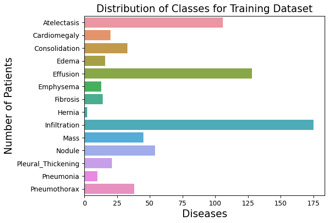
Let's plot this with bars to represent the distribution of classes (pathologies) within the 1000 samples:

label_count = []

for column in columns:
    label_count.append(train_df[column].sum())

sns.barplot(x=label_count, y=columns)
plt.title('Distribution of Classes for Training Dataset', fontsize=15)
plt.ylabel('Number of Patients', fontsize=15)
plt.xlabel('Diseases', fontsize=15)
plt.show()

We can see how Atelectasis, Effusion, and Infiltration are in high counts compared to the other pathologies.

To finish this first section of the data exploration, we only missed the image and how it is connected to this data.

As I mentioned before, the data we got has only the name of the image file, so after downloading the images locally, we can access them in this way:

img_dir = '/images/images-small/'
img = train_df.Image[0]
image = plt.imread(os.path.join(img_dir, img))

plt.imshow(image, cmap='gray')
plt.colorbar()
plt.title('Raw Chest X Ray Image')

print(f"The dimensions of the image are {image.shape[0]} pixels width and {image.shape[1]} pixels height, one single color channel")
print(f"The maximum pixel value is {image.max():.4f} (white) and the minimum is {image.min():.4f} (black)")
print(f"The mean value of the pixels is {image.mean():.4f} and the standard deviation is {image.std():.4f}")

# The dimensions of the image are 1024 pixels width and 1024 pixels height, one single color channel
# The maximum pixel value is 0.9804 (white) and the minimum is 0.0000 (black)
# The mean value of the pixels is 0.4796 and the standard deviation is 0.2757

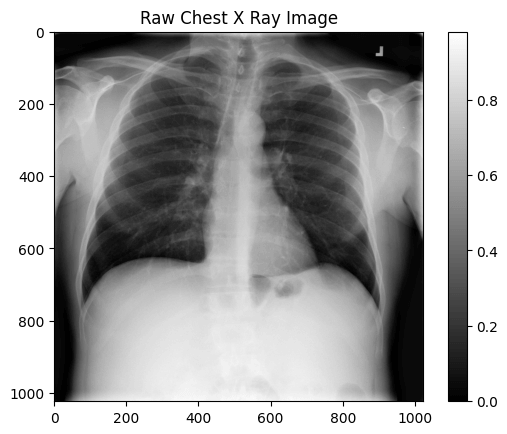
It's an image with a 1024x1024 dimension, black and white.

Before moving to the model development, we should take a look at the data a little bit closer and check if we need to process it before passing it to the model.

Preprocessing: Data Leakage, Image Preprocessing, Class Imbalance

In this section, we will explore how the data is leaked, how to preprocess the images, handle class imbalance, and build the dataset and dataloader.

Starting with data leakage, we are training the model on patient samples, so we don't want to train the model on the training data for one patient, and then test it on the validation and testing sets, where they also have the same patient sample.

Let's first check if there are the same patients among the training, validation, and test sets. We start with this function, checking the intersection of two dataframes:

def check_for_leakage(df1, df2, patient_col):
    return bool(set(df1[patient_col]).intersection(set(df2[patient_col])))

Let's check the intersections:

print(f"Leakeage between train and validation sets: {check_for_leakage(train_df, valid_df, 'PatientId')}")
print(f"Leakeage between train and test sets: {check_for_leakage(train_df, test_df, 'PatientId')}")
print(f"Leakeage between validation and test sets: {check_for_leakage(valid_df, test_df, 'PatientId')}")

# Leakeage between train and validation sets: True
# Leakeage between train and test sets: False
# Leakeage between validation and test sets: False

Apparently, we have leakage between the train the validation sets.

We need to understand how many patients are leaked and what IDs we need to handle:

overlapping_patient_ids = set(train_df["PatientId"]).intersection(set(valid_df["PatientId"]))
num_of_overlaps = len(overlapping_patient_ids)
print(f"Number of unique overlaps between train and validation sets: {num_of_overlaps}")
print(f"These are the overlapping patient IDs: {overlapping_patient_ids}")

# Number of unique overlaps between train and validation sets: 11
# These are the overlapping patient IDs: {20290, 27618, 9925, 10888, 22764, 19981, 18253, 4461, 28208, 8760, 7482}

We have 11 of them between the train and the validation sets. With the IDs, we can remove these samples from the validation set.

print(f"Current validation set shape: {valid_df.shape}")
valid_df = valid_df[~valid_df["PatientId"].isin(overlapping_patient_ids)]
print(f"New validation set shape (without overlapping patients): {valid_df.shape}")

# Current validation set shape: (109, 16)
# New validation set shape (without overlapping patients): (96, 16)

Checking it again, there's no leakage between the train and validation sets anymore.

print(f"Leakeage between train and validation sets: {check_for_leakage(train_df, valid_df, 'PatientId')}")
# Leakeage between train and validation sets: False

If you remember, the training dataset has only 2 samples of Hernia and 10 samples of pneumonia, compared to 128 of Effusion and 175 of Infiltration out of 1000 samples. So, there is a huge class imbalance here.

This imbalance issue can hugely contribute to a poor loss computation: Overwhelms the gradients from the other 13 classes → Forces massive, unstable updates to the model weights → Loss plateau.

In other words, the model won't learn properly.

Soon, I will talk about BCEWithLogitsLoss and how it will be used in the model training, but the important information for now is that it has a parameter called pos_weight, so we can use it to balance the contribution of positive and negative samples. We do this by dividing the negative samples by the positive samples.

label_condition_incidence = pd.DataFrame({"Condition": [], "Positive Count": [], "Negative Count": []})

samples_count = train_df.shape[0]

print(f"Samples count: {samples_count}")
print("===================")

for column in columns:
    positive_label_count = train_df[column].sum()
    negative_label_count = samples_count - positive_label_count
    pos_weight = negative_label_count / positive_label_count
    label_condition_incidence = pd.concat([
        label_condition_incidence,
        pd.DataFrame({
            "Condition": [column],
            "Positive Count": [positive_label_count],
            "Negative Count": [negative_label_count],
            "Pos Weight": [pos_weight]
        })
    ], ignore_index=True)

This is the generated dataframe with all 14 classes, the positive and negative counts, and the pos_weight:

# |    | Condition          |   Positive Count |   Negative Count |   Pos Weight |
# |---:|:-------------------|-----------------:|-----------------:|-------------:|
# |  0 | Atelectasis        |              106 |              894 |     8.4      |
# |  1 | Cardiomegaly       |               20 |              980 |     49       |
# |  2 | Consolidation      |               33 |              967 |     29.3     |
# |  3 | Edema              |               16 |              984 |     61.5     |
# |  4 | Effusion           |              128 |              872 |     6.8      |
# |  5 | Emphysema          |               13 |              987 |     75.9     |
# |  6 | Fibrosis           |               14 |              986 |     70.4     |
# |  7 | Hernia             |                2 |              998 |     499      |
# |  8 | Infiltration       |              175 |              825 |     4.71     |
# |  9 | Mass               |               45 |              955 |     21.2     |
# | 10 | Nodule             |               54 |              946 |     17.5     |
# | 11 | Pleural_Thickening |               21 |              979 |     46.6     |
# | 12 | Pneumonia          |               10 |              990 |     99       |
# | 13 | Pneumothorax       |               38 |              962 |     25.3     |

Some are still pretty big, like Hernia, which has pos_weight of 499. We will handle that later with a simple trick when creating the loss function.

With the data handled, let's focus on the images now. We will use transforms for two things: to preprocess and augment the images.

• Preprocess: resize, transform into tensors, normalize
• Augmentation: rotation, flipping, translation, scaling

Here is the implementation:

transform = transforms.Compose([
    transforms.Resize((320, 320)),
    transforms.RandomHorizontalFlip(),
    transforms.RandomRotation(20),
    transforms.RandomAffine(
        degrees=0,
        translate=(0.2, 0.2),
        scale=(0.8, 1.2),
        shear=20
    ),
    transforms.ToTensor(),
    transforms.Normalize(
        mean=[0.485, 0.456, 0.406],
        std=[0.229, 0.224, 0.225]
    )
])

Let's build our custom dataset now, so we can test this transform.

We should pass the dataframe, the image directory, and the transform for the dataset and it will handle the data for us. The getitem will handle and return the transformed image and the labels.

class CustomImageDataset(Dataset):
    def __init__(self, df, image_dir, transform=None):
        self.df = df
        self.transform = transform
        self.image_dir = image_dir

    def __len__(self):
        return len(self.df)

    def __getitem__(self, index):
        image_name = self.df.iloc[index]["Image"]
        labels = self.df.iloc[index].filter(items=columns)
        labels = torch.tensor(labels, dtype=torch.float32)

        image_path = os.path.join(self.image_dir, image_name)
        image = Image.open(image_path).convert("RGB")

        if self.transform:
            image = self.transform(image)

        return image, labels

If there is a transform, use it for the image. This is also an interesting implementation because we use Image.open per item of the dataset, so only one item image at a time is held in memory.

Now, let's test the transform we built before:

raw_dataset = CustomImageDataset(
    df=train_df,
    image_dir="/kaggle/input/images/images-small/"
)

image, label = raw_dataset[0]

print(f"Raw image: {image.size}")
image = transforms.Resize((320, 320))(image)
print(f"Resized image: {image.size}")
image = transforms.RandomHorizontalFlip()(image)
print(f"Random flipped image: {image.size}")
image = transforms.RandomRotation(20)(image)
print(f"Random rotated image: {image.size}")
image = transforms.RandomAffine(
    degrees=0,
    translate=(0.2, 0.2),
    scale=(0.8, 1.2),
    shear=20
)(image)
print(f"Random affine image: {image.size}")
image = transforms.ToTensor()(image)
print(f"Tensor image: {image.shape}, range[{image.min():.1f}, {image.max():.1f}]")
image = transforms.Normalize(
    mean=[0.485, 0.456, 0.406],
    std=[0.229, 0.224, 0.225]
)(image)
print(f"Normalized image: {image.shape}, range[{image.min():.1f}, {image.max():.1f}]")

# Raw image: (1024, 1024)
# Resized image: (320, 320)
# Random flipped image: (320, 320)
# Random rotated image: (320, 320)
# Random affine image: (320, 320)
# Tensor image: torch.Size([3, 320, 320]), range[0.0, 0.9]
# Normalized image: torch.Size([3, 320, 320]), range[-2.1, 2.3]

We can see the transformations one by one. This is also useful as a debugging technique to make sure we are preprocessing and augmenting the images properly.

To end this part, we should create a dataloader, where we will shuffle the data and divide the items into batches.

dataloader = DataLoader(
    dataset,
    batch_size=64,
    shuffle=True
)

Let's test it:

data_iter = iter(dataloader)
batch = next(data_iter)
images, labels = batch
images.shape # torch.Size([64, 3, 320, 320])
labels.shape # torch.Size([64, 14])

64 is the size of each batch. The image is an RGB image, so 3 channels, with a 320x320 dimension. The label also has the same 64 size for the batch, and 14 labels, or pathologies.

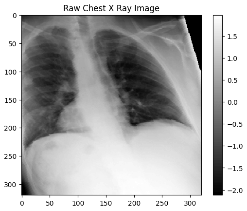
Getting one image and exploring it, we can see its properties:

transformed_image = images[0]

plt.imshow(transformed_image[0], cmap='gray')
plt.colorbar()
plt.title('Raw Chest X Ray Image')
print(transformed_image.shape)
print(f"The dimensions of the transformed_image are {transformed_image.shape[1]} pixels width and {transformed_image.shape[2]} pixels height")
print(f"The maximum pixel value is {transformed_image.max():.4f} and the minimum is {transformed_image.min():.4f}")
print(f"The mean value of the pixels is {transformed_image.mean():.4f} and the standard deviation is {transformed_image.std():.4f}")

# torch.Size([3, 320, 320])
# The dimensions of the transformed_image are 320 pixels width and 320 pixels height
# The maximum pixel value is 2.3611 and the minimum is -2.1179
# The mean value of the pixels is 0.3880 and the standard deviation is 1.1588

Model Development & Model Training

For the model architecture, we will build a simple CNN just to test it on the data and see how it performs.

This model has 4 convolution layers with ReLU and pooling layers, then it uses fully connected layers with dropout, reducing it to 14 probabilities.

class XRayCNN(nn.Module):
    def __init__(self):
        super(XRayCNN, self).__init__()
        self.conv1 = nn.Conv2d(in_channels=3, out_channels=16, kernel_size=3, padding=1)
        self.conv2 = nn.Conv2d(in_channels=16, out_channels=32, kernel_size=3, padding=1)
        self.conv3 = nn.Conv2d(in_channels=32, out_channels=64, kernel_size=3, padding=1)
        self.conv4 = nn.Conv2d(in_channels=64, out_channels=128, kernel_size=3, padding=1)
        self.pool = nn.MaxPool2d(2, 2)
        # flattening the 3d structure: 128 (Channels) * 20 (Height) * 20 (Width)
        self.fc1 = nn.Linear(128 * 20 * 20, 1024)
        self.dropout = nn.Dropout(0.25)
        # 14 pathology classes
        self.fc2 = nn.Linear(1024, 14)

    def forward(self, x):
        x = self.pool(relu(self.conv1(x)))
        x = self.pool(relu(self.conv2(x)))
        x = self.pool(relu(self.conv3(x)))
        x = self.pool(relu(self.conv4(x)))
        x = x.view(-1, 128 * 20 * 20)
        x = self.fc1(x)
        x = self.dropout(x)
        x = self.fc2(x)
        return x

Let's unwrap how it is implemented.

We need to recap the equations of convolution and max pooling.

Convolution: $Hout=[(Hin−K+2P)/S]+1$

MaxPooling: $Hout=[(Hin−K)/S]+1$

• $Hin$ = Input Height/Width
• $K$ = kernel_size (3 for all conv layers)
• $P$ = padding (1 for all conv layers)
• $S$ = stride (defaults to 1 for all conv layers)

Applying these equations for all the layers, we get:

Shape: (3, 320, 320)

• Conv1: $320=[(320−3+2∗1)/1]+1$
• Pool1: $160=[(320−2)/2]+1$
• Conv2: $160=[(160−3+2∗1)/1]+1$
• Pool2: $80=[(160−2)/2]+1$
• Conv3: $80=[(80−3+2∗1)/1]+1$
• Pool3: $40=[(80−2)/2]+1$
• Conv4: $40=[(40−3+2∗1)/1]+1$
• Pool4: $20=[(40−2)/2]+1$

The final output of the convolution layer is (B, 128, 20, 20)

• $C=128$
• $H=20$
• $W=20$

In the fully connected layers, we need a 1-dimensional input. This is why we flatten it. To flatten it, we need to multiply all the dimensions: $128 \cdot 20 \cdot 20$.

With that model, we can start training it and see how it performs.

First, let's build the loss, the metrics, and the optimizer.

Here are the metrics:

def compute_metrics(targets, probs, threshold=0.5):
    y_score = (probs >= threshold).astype(int)
    roc_auc_class = roc_auc_score(targets, probs, average=None)
    roc_auc_mean = np.mean(roc_auc_class)

    return {
        "accuracy": accuracy_score(targets, y_score),
        "precision": precision_score(targets, y_score, average=None),
        "recall": recall_score(targets, y_score, average=None),
        "roc_auc_per_class": roc_auc_class,
        "roc_auc_mean": roc_auc_mean
    }

We will measure accuracy, precision, recall, ROC AUC per class, and ROC AUC mean.

For the optimizer, we have Adam:

optimizer = optim.Adam(model.parameters(), lr=0.0001)

For the loss function, we will use BCEWithLogitsLoss that I mentioned before and use the computed pos weight that is stored in label_condition_incidence.

Remember that some weight values are very high. To reduce those weights, we will ‘clamp’ them using the square root:

pos_weight = torch.sqrt(torch.tensor(label_condition_incidence["Pos Weight"]))
loss_function = nn.BCEWithLogitsLoss(pos_weight=pos_weight)

With all these implemented, we can train our model.

We run the model for 25 epochs, compute the loss and the metrics, store them so we can plot them later, and print them in each epoch for debugging purposes.

model = XRayCNN()
num_epochs = 25
loss_history = []
accuracy_history = []
roc_auc_history = []

for epoch in range(num_epochs):
    model.train()
    running_loss = 0.0
    all_targets = []
    all_probs = []

    for images, labels in dataloader:
        optimizer.zero_grad()
        output = model(images)
        probs = torch.sigmoid(output)
        all_targets.append(labels.detach().numpy())
        all_probs.append(probs.detach().numpy())
        loss = loss_function(output, labels)
        running_loss += loss
        loss.backward()
        optimizer.step()

    epoch_loss = running_loss / len(dataloader)
    loss_history.append(epoch_loss.item())
    print(f"Epoch {epoch + 1}")
    print("==================")
    print(f"Loss: {epoch_loss:.4f}")

    y_true = np.concatenate(all_targets, axis=0)
    y_score = np.concatenate(all_probs, axis=0)
    model_metrics = compute_metrics(y_true, y_score)
    accuracy_history.append(model_metrics['accuracy'])
    roc_auc_history.append(model_metrics['roc_auc_mean'])

    print(f"accuracy: {model_metrics['accuracy']}")
    print(f"roc_auc_mean: {model_metrics['roc_auc_mean']}")

This is what we get from printing each epoch:

Epoch 1
==================
Loss: 0.5352
accuracy: 0.522
roc_auc_mean: 0.48672466487573834

Epoch 2
==================
Loss: 0.4899
accuracy: 0.562
roc_auc_mean: 0.5037439466896264

Let's plot the graphs for the loss, accuracy, and roc_auc_mean over the epochs.

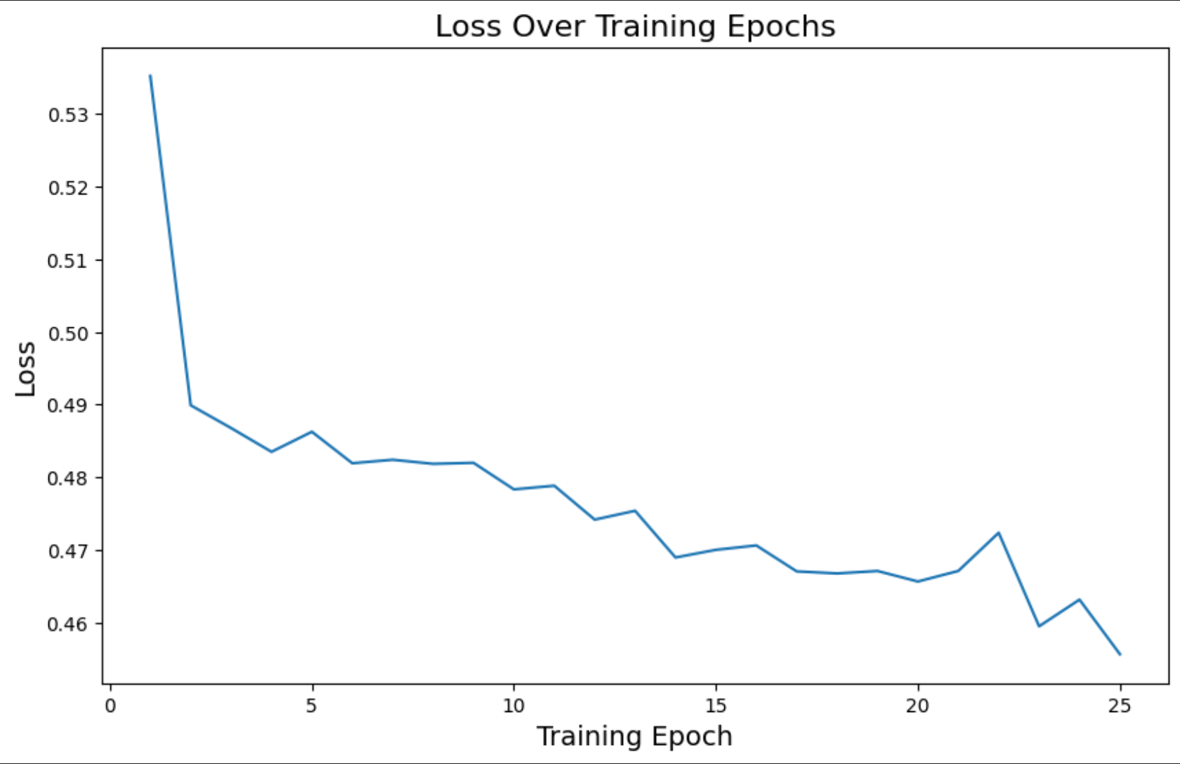
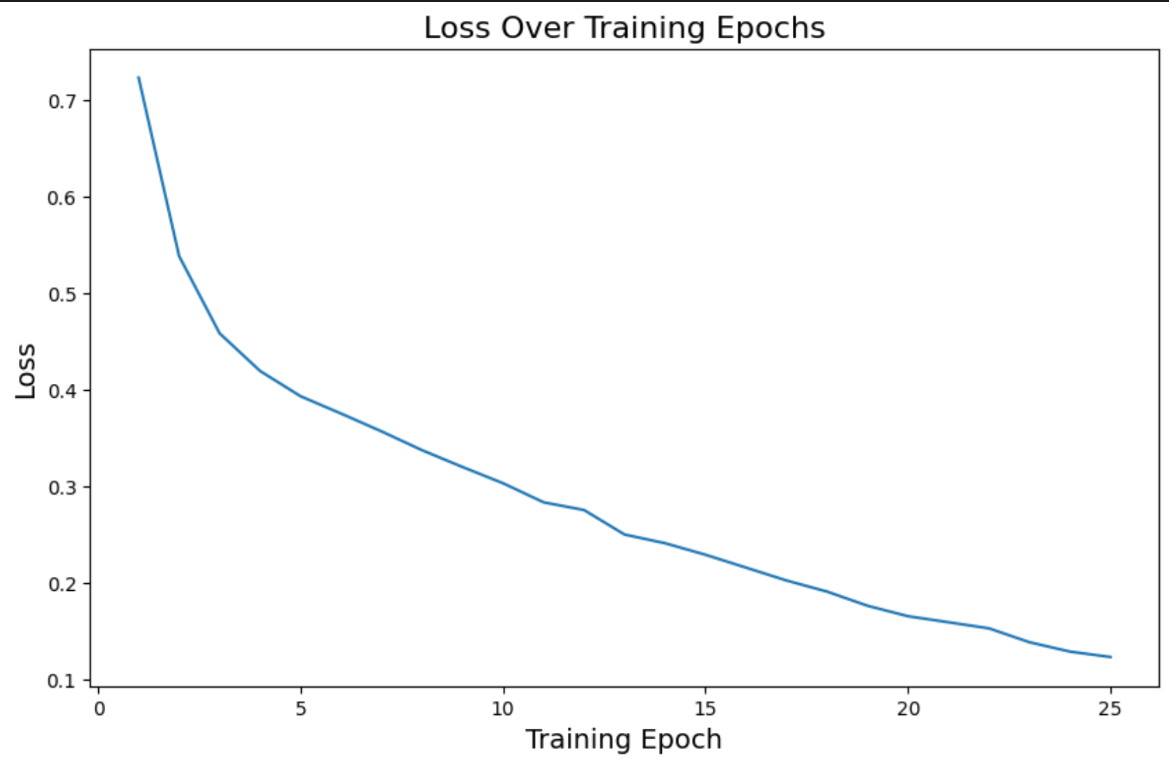
Loss

epochs = list(range(1, num_epochs + 1))
loss_history = [loss for loss in loss_history]

plt.figure(figsize=(10, 6))
plt.plot(epochs, loss_history)
plt.title('Loss Over Training Epochs', fontsize=16)
plt.xlabel('Training Epoch', fontsize=14)
plt.ylabel('Loss', fontsize=14)
plt.show()

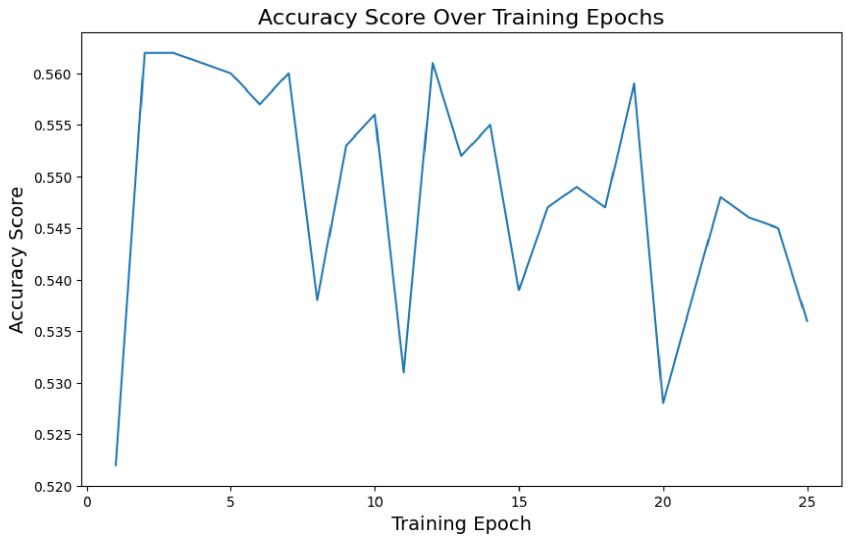
Accuracy

plt.figure(figsize=(10, 6))
plt.plot(epochs, accuracy_history)
plt.title('Accuracy Score Over Training Epochs', fontsize=16)
plt.xlabel('Training Epoch', fontsize=14)
plt.ylabel('Accuracy Score', fontsize=14)
plt.show()

ROC AUC mean

plt.figure(figsize=(10, 6))
plt.plot(epochs, roc_auc_history)
plt.title('ROC AUC Score Over Training Epochs', fontsize=16)
plt.xlabel('Training Epoch', fontsize=14)
plt.ylabel('ROC AUC Score', fontsize=14)
plt.show()

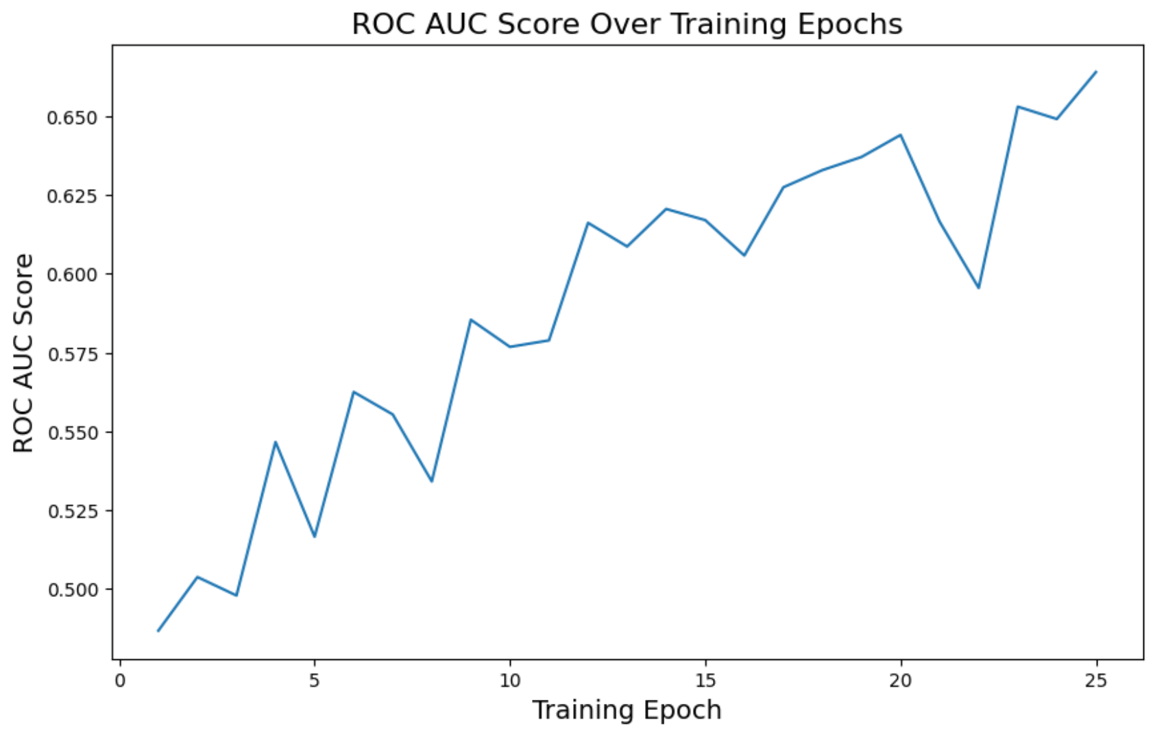
The loss decreased over time as expected, and ROC AUC improved a bit, but accuracy was too unstable.

Loss reached 0.45. Accuracy went to 0.53, and ROC AUC 0.66. In other words, not that great.

We could experiment with other architectures and adjust the current model, but I wanted to try using Transfer Learning and test it on this dataset.

Another important thing to note here is that I tried using the actual pos_weight that was calculated but the loss never decreased. This is why it was important to clamp it using square root.

Transfer Learning with ResNet

For transfer learning, we will be using ResNet18, a Deep Residual Learning model trained on ImageNet. After this base model, we apply a fully connected layer to output the expected number of probability classes (14) for our problem.

from torchvision import models

class TransferLearningXRay(nn.Module):
    def __init__(self, num_classes=14):
        super(TransferLearningXRay, self).__init__()
        self.base_model = models.resnet18(pretrained=True)
        in_features = self.base_model.fc.in_features
        self.base_model.fc = nn.Linear(in_features, num_classes)

    def forward(self, x):
        return self.base_model(x)

Let's train it with a similar implementation for the previous model.

loss_function = nn.BCEWithLogitsLoss(pos_weight=pos_weight)
model = TransferLearningXRay()
optimizer = optim.Adam(model.parameters(), lr=0.0001)
num_epochs = 25
loss_history = []
accuracy_history = []
roc_auc_history = []

for epoch in range(num_epochs):
    model.train()
    running_loss = 0.0
    all_targets = []
    all_probs = []

    for images, labels in dataloader:
        optimizer.zero_grad()
        output = model(images)
        probs = torch.sigmoid(output)
        all_targets.append(labels.detach().numpy())
        all_probs.append(probs.detach().numpy())
        loss = loss_function(output, labels)
        running_loss += loss
        loss.backward()
        optimizer.step()

    epoch_loss = running_loss / len(dataloader)
    loss_history.append(epoch_loss.item())
    y_true = np.concatenate(all_targets, axis=0)
    y_score = np.concatenate(all_probs, axis=0)
    model_metrics = compute_metrics(y_true, y_score)
    accuracy_history.append(model_metrics['accuracy'])
    roc_auc_history.append(model_metrics['roc_auc_mean'])

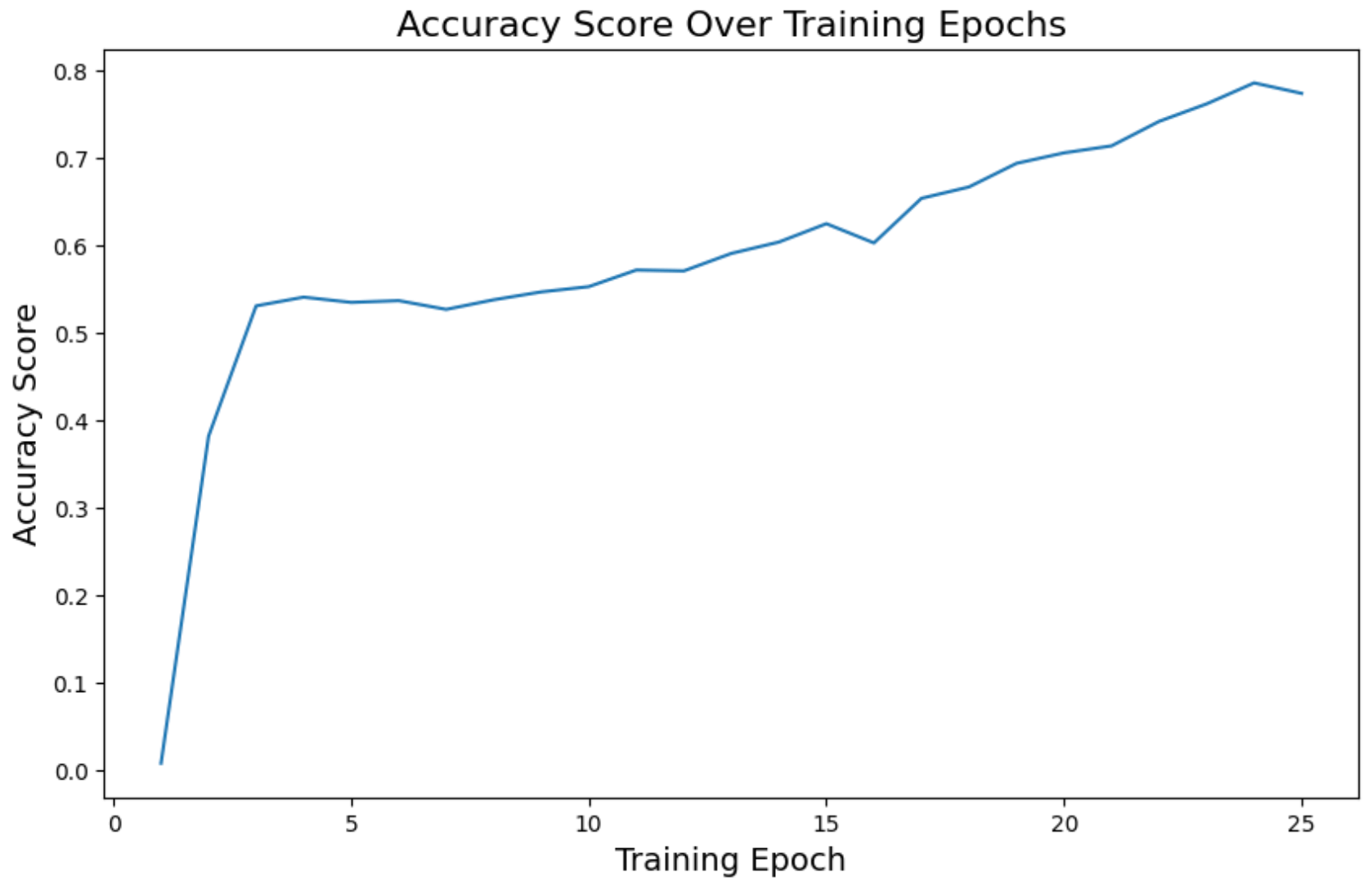
On the last epoch, we have these metrics:

• loss: 0.12
• accuracy: 0.77
• roc_auc_mean: 0.98

Much better compared to the other model predictions.

Loss

Accuracy

ROC AUC

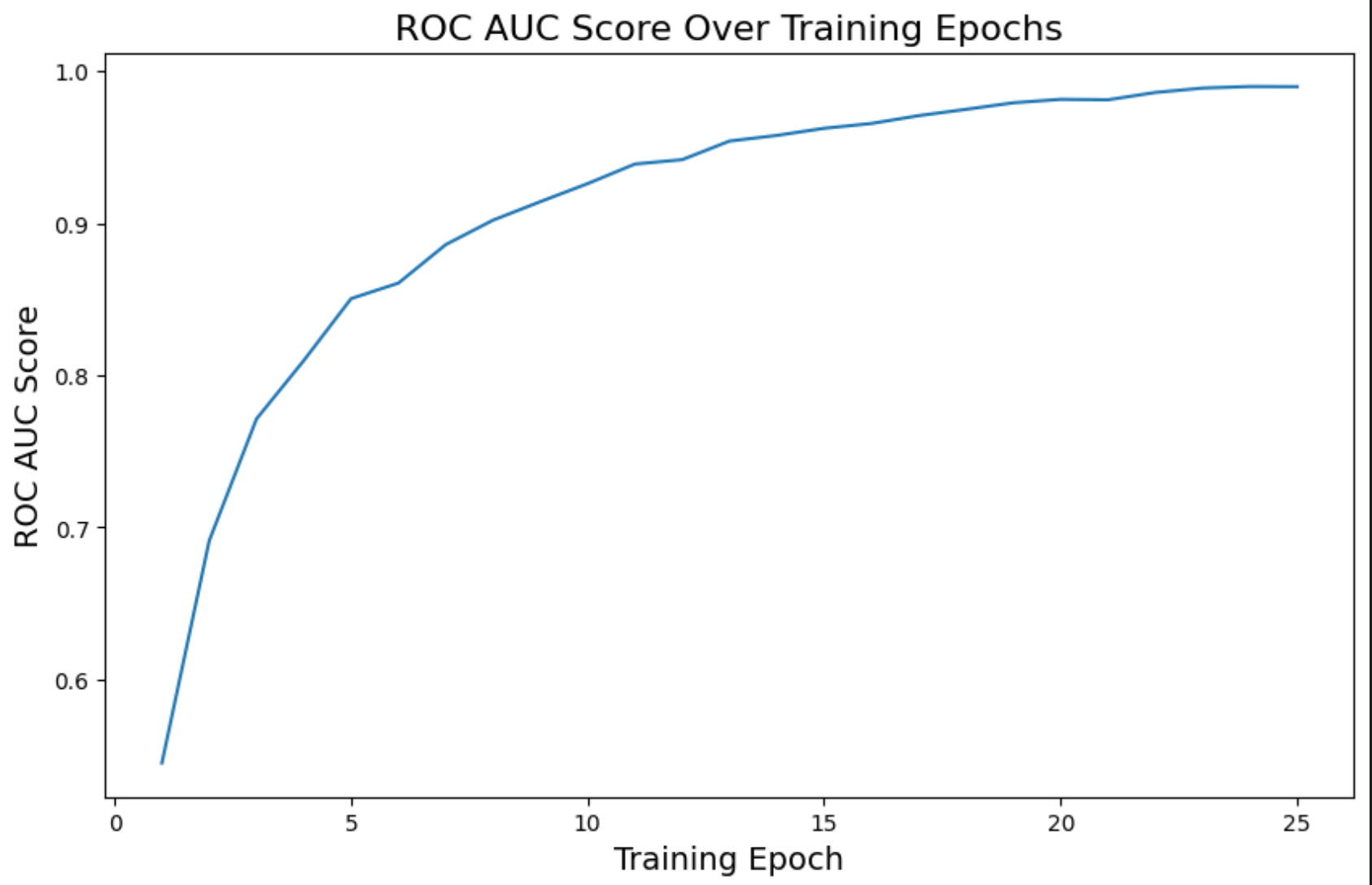
We can see how these metrics are a much better and improved version compared to the other model.

Going Deeper

This was a simple project to test out some of the things I learned using PyTorch, so there are a lot of things that can be improved here. Some ideas for a future version of this project:

• Use a GPU device and measure how much faster the training gets, especially when training on ResNet
• Divide the problem into different classes, so we can have separate accuracy, precision, ROC AUC, and other metrics for each class
• Test different thresholds to measure the metrics. This version is currently using 0.5 as a threshold
• Test new architectures for the first model: adding more convolution layers, understanding where it's failing to learn, experimenting with residual blocks, etc
• Do some tests on the validation and test sets to see if the model is generalizing

There is a ton of stuff we can do to keep learning and trying new things. But I hope this blogpost is enough to show some small ideas for this specific problem.

Resources

• Chest X-Ray Medical Diagnosis with Deep Learning
• Mastering PyTorch: From Linear Regression to Computer Vision
• Machine Learning Research
• AI/ML for Biology & Healthcare: A Learning Path

Twitter · Github