Deep Learning for Biology: Predicting Protein Functions from Sequences
 Photo by Adrian Siaril
This month, I started reading the Deep Learning for Biology book and working on protein prediction, so I can get a sense of biology data, biology challenges, and how to leverage ML for these kinds of problems.
In this piece, I want to share the learnings I gained from the first chapter, where I implemented a model to predict protein functions based on their sequences.
Here is what we are going to cover:
- What are proteins?
- The problem of predicting protein functions
- Why predict protein functions?
- Large Language Models (LLMs) & Embeddings
- Extracting an Embedding for an Entire Protein
- Predicting protein function
Here we go!
What are proteins?
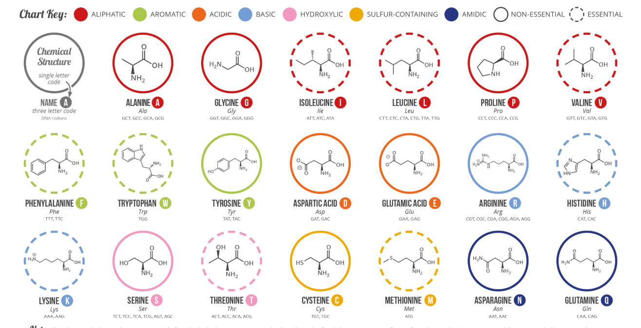
According to NCI, a protein is a molecule made up of amino acids that are needed for the body to function properly. It's a building block with a sequence of 20 amino acids. Each type of protein has a different structure, role, and function.
One example is insulin, a protein hormone that signals cells to absorb sugar from the bloodstream.
Understanding the protein structure is crucial because it directly influences the protein function. It's described in four hierarchical levels:
- Primary structure*:* The linear sequence of amino acids
- Secondary structure*:* Local folding into structural elements such as alpha helices and beta sheets
- Tertiary structure*:* The overall 3D shape formed by the complete amino acid chain
- Quaternary structure*:* The assembly of multiple protein subunits into a functional complex
In terms of protein functions, we can categorize them into 3 types:
- Biological process: This contributes to cell division, response to stress, carbohydrate metabolism, or immune signaling.
- Molecular function: This describes the specific biochemical activity of the protein itself—such as binding to DNA or ATP (a molecule that stores and transfers energy in cells), acting as a kinase (an enzyme that attaches a small chemical tag called a phosphate group to other molecules to change their activity), or transporting ions across membranes.
- Cellular component: This indicates where in the cell the protein usually resides—such as the nucleus, mitochondria, or extracellular space. Although it’s technically a location label and not a function per se, it often provides important clues about the protein’s role (e.g., proteins in the mitochondria are probably involved in energy production).
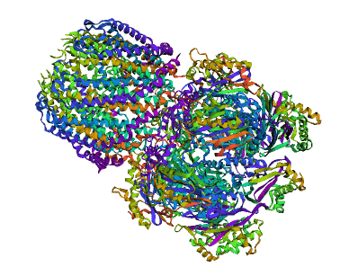
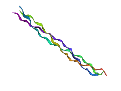
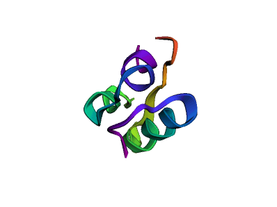
Now that we understand the importance of proteins and how they work, let's visualize their structure using the Py3Dmol library.
import py3Dmol
import requests

def fetch_protein_structure(pdb_id: str) -> str:
  """Grab a PDB protein structure from the RCSB Protein Data Bank."""
  url = f"https://files.rcsb.org/download/{pdb_id}.pdb"
  return requests.get(url).text

protein_to_pdb = {
  "insulin": "3I40",  # Human insulin – regulates glucose uptake.
  "collagen": "1BKV",  # Human collagen – provides structural support.
  "proteasome": "1YAR",  # Archaebacterial proteasome – degrades proteins.
}

protein = "proteasome"
pdb_structure = fetch_protein_structure(pdb_id=protein_to_pdb[protein])

pdbview = py3Dmol.view(width=400, height=300)
pdbview.addModel(pdb_structure, "pdb")
pdbview.setStyle({"cartoon": {"color": "spectrum"}})
pdbview.zoomTo()
pdbview.show()
This code will plot different protein structures: insulin, collagen, and proteasome. It basically requests the RCSB Protein Data Bank dataset and gets the protein structure to be plotted via Py3Dmol, so we can see the structure in 3D.
Before moving to the protein function prediction problem, let's see how proteins are represented. As we learned before, proteins are long chains of amino acids. There are 20 different types of amino acids that combine to create the vast array of proteins.
To let machine learning models read this type of data, we need their numerical representation.
We use one-hot encoding to build this numerical representation. Because we have 20 standard amino acids, for each amino acid, we should have one vector of 20 positions, where each position represents each specific amino acid.
If the position has a value of 1, it means it's the amino acid in question. The other positions will be placed as 0.
Let's build these one-hot encoding numerical representations.
First, we need to create a list of all amino acids:
amino_acids = [
  "R", "H", "K", "D", "E",
  "S", "T", "N", "Q", "G",
  "P", "C", "A", "V", "I",
  "L", "M", "F", "Y", "W",
]
Then, we need to build the id or index for each amino acid.
amino_acid_to_index = {
  amino_acid: index for index, amino_acid in enumerate(amino_acids)
}
We'll use the array index as its numerical representation. The amino_acid_to_index will hold the amino acid letter as the key and the index as the value of the map. Like this:
{'R': 0, 'H': 1, 'K': 2} # etc
Now, let's take a small protein sequence:
# Methionine, alanine, leucine, tryptophan, methionine.
tiny_protein = ["M", "A", "L", "W", "M"]
And build its numerical representation.
tiny_protein_indices = [
  amino_acid_to_index[amino_acid] for amino_acid in tiny_protein
]

# [16, 12, 15, 19, 16]
The output vector will hold all the indices for each amino acid.
With that in mind, we can use it to build the one-hot encoding numerical version of the protein.
We'll use JAX’s one_hot function to do this:
import jax

one_hot_encoded_sequence = jax.nn.one_hot(
  x=tiny_protein_indices, num_classes=len(amino_acids)
)

# [[0. 0. 0. 0. 0. 0. 0. 0. 0. 0. 0. 0. 0. 0. 0. 0. 1. 0. 0. 0.]
#  [0. 0. 0. 0. 0. 0. 0. 0. 0. 0. 0. 0. 1. 0. 0. 0. 0. 0. 0. 0.]
#  [0. 0. 0. 0. 0. 0. 0. 0. 0. 0. 0. 0. 0. 0. 0. 1. 0. 0. 0. 0.]
#  [0. 0. 0. 0. 0. 0. 0. 0. 0. 0. 0. 0. 0. 0. 0. 0. 0. 0. 0. 1.]
#  [0. 0. 0. 0. 0. 0. 0. 0. 0. 0. 0. 0. 0. 0. 0. 0. 1. 0. 0. 0.]]
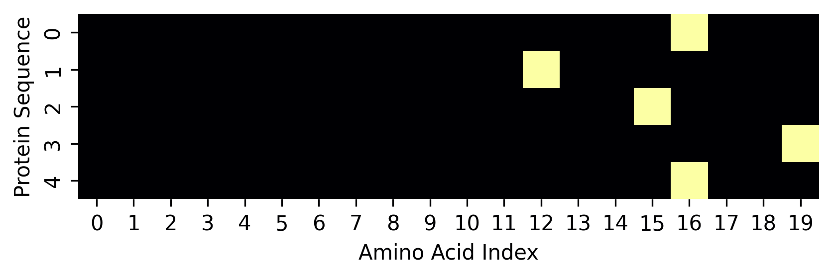
The tiny_protein has 5 amino acids, so the vector holds 5 other vectors. Each inner vector has 0s and 1, describing which amino acid this vector represents.
Take the first inner vector. It has 0 in all positions, but position 16, where it holds a value 1, describing it as a methionine amino acid.
We can also represent this one-hot encoding representation as an image. Take the same output and let's plot it as an image using seaborn.
import seaborn as sns

fig = sns.heatmap(
  one_hot_encoded_sequence, square=True, cbar=False, cmap="inferno"
)
fig.set(xlabel="Amino Acid Index", ylabel="Protein Sequence");
The problem of predicting protein functions
As we saw before, a protein sequence describes its 3D structure, which determines its biological function.
The problem of predicting protein functions is a big challenge in biology. In this post, we'll see how to use ML to predict these biological functions using neural networks and pretrained embeddings.
But before that, let's see what is the actual problem.
To train a ML model to predict protein functions, we need to give it the sequence and expect it to output the probabilities of all possible functions. Let's see the following examples:
- Given the sequence of the
COL1A1collagen protein (MFSFVDLR...), we might predict its function is likelystructuralwith probability 0.7,enzymaticwith probability 0.01, and so on. - Given the sequence of the
INSinsulin protein (MALWMRLL...), we might predict its function is likelymetabolicwith probability 0.6,signalingwith probability 0.3, and so on.
The COL1A1 protein has a high probability of having a structural function. While the INS protein with a high probability of a metabolic function.
Why Predict Protein Functions?
Before moving on to the prediction algorithm, let's just take a look at why we do protein function prediction.
Proteins are building blocks of biology, and solving this problem would open new opportunities in the whole field.
In general, with ML, we can have better protein function hypothesis (better classification) for unknown functions, we can better understand how diseases work, and design and engineer therapeutic proteins for medicine.
The book goes deeper into these reasons:
- Biotechnology and protein engineering: If we can reliably predict function from sequence, we can begin to design new proteins with desired properties. This could be useful for designing enzymes for industrial chemistry, therapeutic proteins for medicine, or synthetic biology components.
- Understanding disease mechanisms: Many diseases are caused by specific sequence changes (variants or mutations) that disrupt protein function. A good predictive model can help identify how specific mutations alter function, offering insights into disease mechanisms and potential therapeutic targets.
- Genome annotation: As we continue sequencing the genomes of new species, we’re uncovering vast numbers of proteins whose functions remain unknown. For newly identified proteins—especially those that are distantly evolutionarily related to any known ones—computational prediction is essential for assigning functional hypotheses.
- Metagenomics and microbiome analysis: When sequencing entire microbial communities, such as gut bacteria or ocean microbiota, many protein-coding genes have no close matches in existing databases. Predicting function from sequence helps uncover the roles of these unknown proteins, advancing our understanding of microbial ecosystems and their effects on hosts or the environment.
Large Language Models (LLMs) & Embeddings
LLMs are trained to predict the next token and have contextual reasoning so that they can output the next character or word and generate entire sentences, such as in text summarization, language translation, and creative writing.
Biology is like language in some ways. DNA and proteins are sequences of characters, which are represented in three-dimensional structures, holding complex patterns. Because we can extract meaning and patterns from sequences and contextual tokens from proteins and DNA, language models can also be useful in biology.
One common representation that is output from an LLM is called an embedding.
An embedding is a numerical vector — a list of floating-point numbers — that encodes the meaning or structure of an input.
A numerical vector example is like this:
[0.2, 0.1, 0.3, 0.2, 0.1, 0.4]
In language models, embeddings are not just numbers, but similar inputs lead to similar embeddings. For language, the model will learn, for example, the “semantic code”, and the embeddings with similar meanings will be placed together in the latent space based on these patterns.
For protein language models, proteins with similar structure or function will be placed closer in the protein space. For example, collagen I and collagen II embeddings will be very close as they have similar “meaning”. We'll see in practice how proteins with the same structures and functions are close together in the latent space.
So these embedding vectors are not only numerical values, but they also hold meaning.
To show how embeddings can be helpful, let's use a pretrained protein language model called ESM2 (paper), developed by Meta. We'll see how the embedding output from the model can hold meaningful information about amino acids.
First, we'll explore the tokenizer and its vocabulary, and test it for a custom sequence of amino acids to see how it represents the protein.
from transformers import AutoTokenizer, EsmModel

model_checkpoint = "facebook/esm2_t33_650M_UR50D"
tokenizer = AutoTokenizer.from_pretrained(model_checkpoint)
The tokenizer is imported from the transformers library. Let's explore the vocabulary it uses:
vocab_to_index = tokenizer.get_vocab()
vocab_to_index
# {'<cls>': 0, '<pad>': 1, '<eos>': 2, '<unk>': 3, 'L': 4, 'A': 5, 'G': 6, 'V': 7, 'S': 8, 'E': 9}
Each token will be represented by a numerical value, similar to what we saw before.
For a protein with this chain of amino acids MALWM, let's see how it will be represented:
tokenized_protein = tokenizer("MALWM")["input_ids"]
tokenized_protein # [0, 20, 5, 4, 22, 20, 2]
As we've seen the vocabulary, we have 33 possible amino acids for this pretrained model. Now, we'll use the pretrained model to get the learned embedding.
token_embeddings = model.get_input_embeddings().weight.detach().numpy()
token_embeddings.shape # (33, 1280)
33 amino acids embedded into a 1280-dimensional space. It's unfeasible for humans to visualize this space, so we'll use dimensionality reduction to visualize it and get an intuition of how embeddings learn patterns and hold meaning.
We'll be using t-SNE to reduce the dimensionality and visualize the embedding patterns.
import pandas as pd
from sklearn.manifold import TSNE

tsne = TSNE(n_components=2, random_state=42)
embeddings_tsne = tsne.fit_transform(token_embeddings)
embeddings_tsne_df = pd.DataFrame(
  embeddings_tsne, columns=["first_dim", "second_dim"]
)
embeddings_tsne_df.shape # (33, 2)
Now we have a 2-dimensional embedding, but still with the 33 amino acids.
Plotting this data, we can see how it is distributed:
fig = sns.scatterplot(
  data=embeddings_tsne_df, x="first_dim", y="second_dim", s=50
)
fig.set_xlabel("First Dimension")
fig.set_ylabel("Second Dimension");
But still, it looks like just a numerical value distribution:
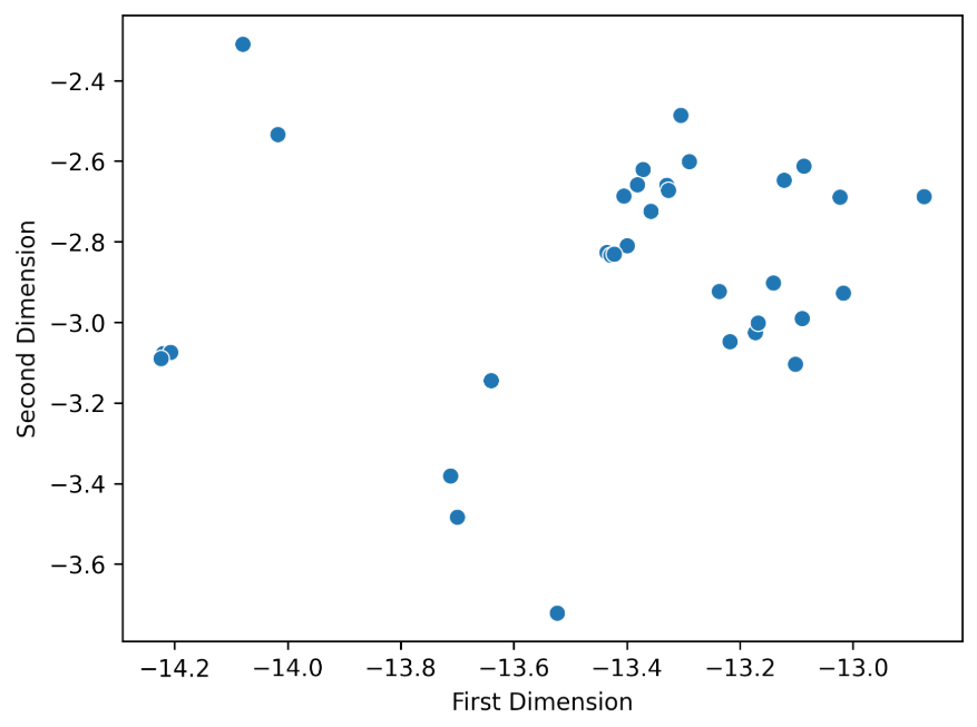
We can see the distribution, but still lack the understanding of patterns and meaning.
To give meaning to this chart, we need to know what each point represents (which amino acid) and see how they are categorized.
Let's start with the categorization:
token_annotation = {
  "hydrophobic": ["A", "F", "I", "L", "M", "V", "W", "Y"],
  "polar uncharged": ["N", "Q", "S", "T"],
  "negatively charged": ["D", "E"],
  "positively charged": ["H", "K", "R"],
  "special amino acid": ["B", "C", "G", "O", "P", "U", "X", "Z"],
  "special token": [
    "-",
    ".",
    "<cls>",
    "<eos>",
    "<mask>",
    "<null_1>",
    "<pad>",
    "<unk>",
  ],
}
We have six categories for all the amino acids. Now we need to build the dataframe to have the tokens (amino acids) and the labels (categories), so we can plot it.
embeddings_tsne_df["token"] = list(vocab_to_index.keys())

embeddings_tsne_df["label"] = embeddings_tsne_df["token"].map(
  {t: label for label, tokens in token_annotation.items() for t in tokens}
)
With that, let's plot the data.
fig = sns.scatterplot(
  data=embeddings_tsne_df,
  x="first_dim",
  y="second_dim",
  hue="label",
  style="label",
  s=50,
)
fig.set_xlabel("First Dimension")
fig.set_ylabel("Second Dimension")
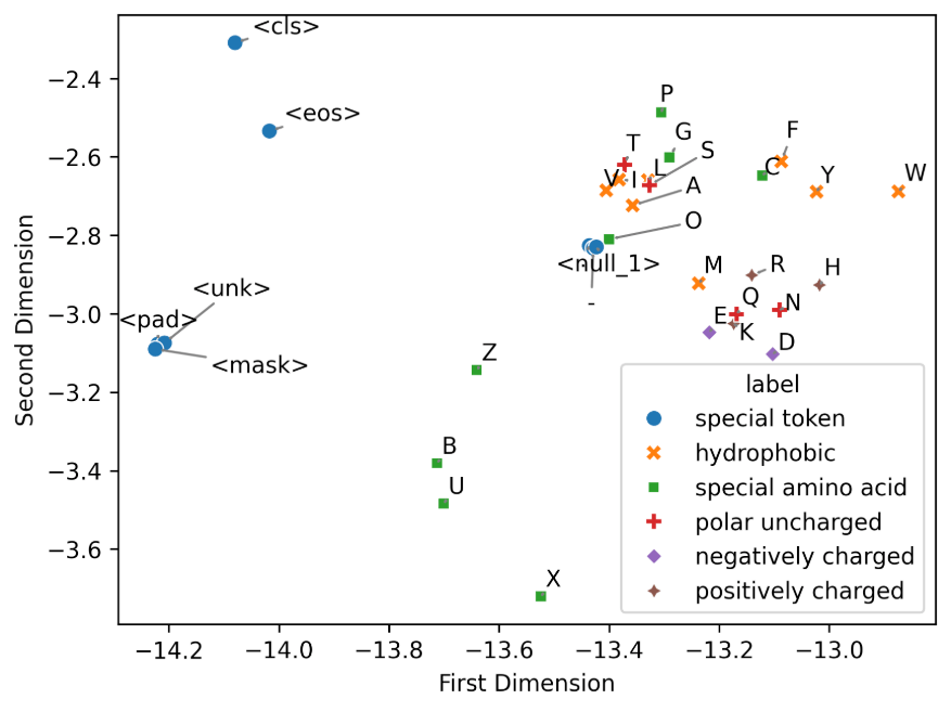
Amino acids with similar (biochemical) properties tend to be placed together. We can see different clusters in the chart. Special amino acids are the green ones, and they are clustered together into two regions. F, Y, and W amino acids are categorized as hydrophobic and also clustered together.
That's the fascinating part of transformer models and their embedding outputs. They have the power to extract patterns and meaning from the input data.
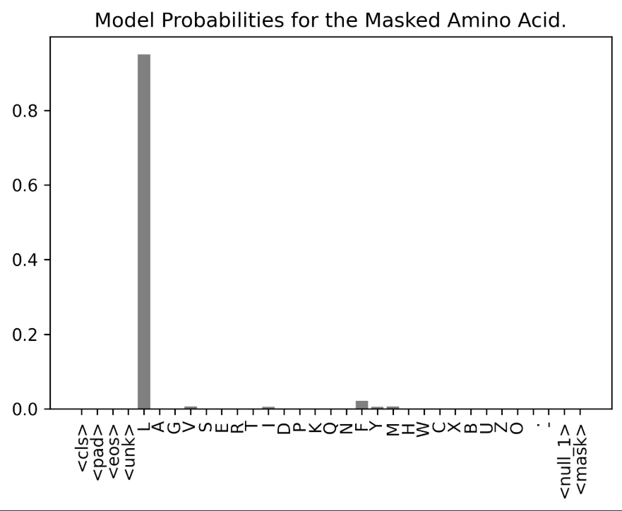
Similar to what LLMs are trained, we'll see how the ESM model predicts masked inputs. Or in this case, masked amino acids in protein sequences.
insulin_sequence = (
  "MALWMRLLPLLALLALWGPDPAAAFVNQHLCGSHLVEALYLVCGERGFFYTPKTRREAEDLQVGQVELGG"
  "GPGAGSLQPLALEGSLQKRGIVEQCCTSICSLYQLENYCN"
)
This is the original protein sequence. Now, we have the masked input:
masked_insulin_sequence = (
  "MALWMRLLPLLALLALWGPDPAAAFVNQH<mask>CGSHLVEALYLVCGERGFFYTPKTRREAEDLQVGQVELGG"
  "GPGAGSLQPLALEGSLQKRGIVEQCCTSICSLYQLENYCN"
)
It's using the <mask> special token in the place of a L amino acid token. This is what the model will try to predict based on the sequence.
Let's instantiate the pretrained model:
from transformers import EsmForMaskedLM

model_checkpoint = "facebook/esm2_t30_150M_UR50D"
tokenizer = AutoTokenizer.from_pretrained(model_checkpoint)
masked_lm_model = EsmForMaskedLM.from_pretrained(model_checkpoint)
And then we can use it to make the prediction:
model_outputs = masked_lm_model(
  **tokenizer(text=masked_insulin_sequence, return_tensors="pt")
)
model_preds = model_outputs.logits
mask_preds = model_preds[0, 30].detach().numpy()
mask_probs = jax.nn.softmax(mask_preds)
We tokenize the sequence and pass it to the model. The model output will hold the prediction in logits. And then, we extract the prediction for the mask position on index 30.
Finally, we apply softmax to get the probabilities. Let's plot the prediction:
import matplotlib.pyplot as plt

letters = list(vocab_to_index.keys())
fig, ax = plt.subplots(figsize=(6, 4))
plt.bar(letters, mask_probs, color="grey")
plt.xticks(rotation=90)
plt.title("Model Probabilities for the Masked Amino Acid.");
The visualization demonstrates the model’s accuracy in predicting the correct amino acid token. This shows how the model learns the structural properties of sequences and the impact of the context of the surrounding amino acids to predict the most probable token.
Extracting an Embedding for an Entire Protein
Before, we predicted a masked amino acid token, and learned how the model learns the context and the surrounding tokens to better predict the actual token.
Now, we want to go further and turn a sequence of amino acids into a single embedding vector, so it captures the protein's overall structure and meaning.
With this embedding representing the patterns and representations of proteins, we can use it as input to predict protein functions based on the protein sequence.
One approach to extract meaning for an entire protein is to use the contextual sequence embeddings from ESM2.
We do this by extracting the final hidden layer activations, which output a vector of (L, D) shape, where L is the number of tokens (amino acids) and D is the model hidden size.
With the last layer vector, we compute the mean pooling and output an embedding with shape (D,). It means that we are averaging all tokens (or amino acids in this case) into a value for each column. The average of these token embeddings is the protein sequence representation.
Averaging seems simplistic, but because the model has already integrated contextual information into each token’s representation using self-attention, the pooled vector still captures meaningful dependencies across the sequence.
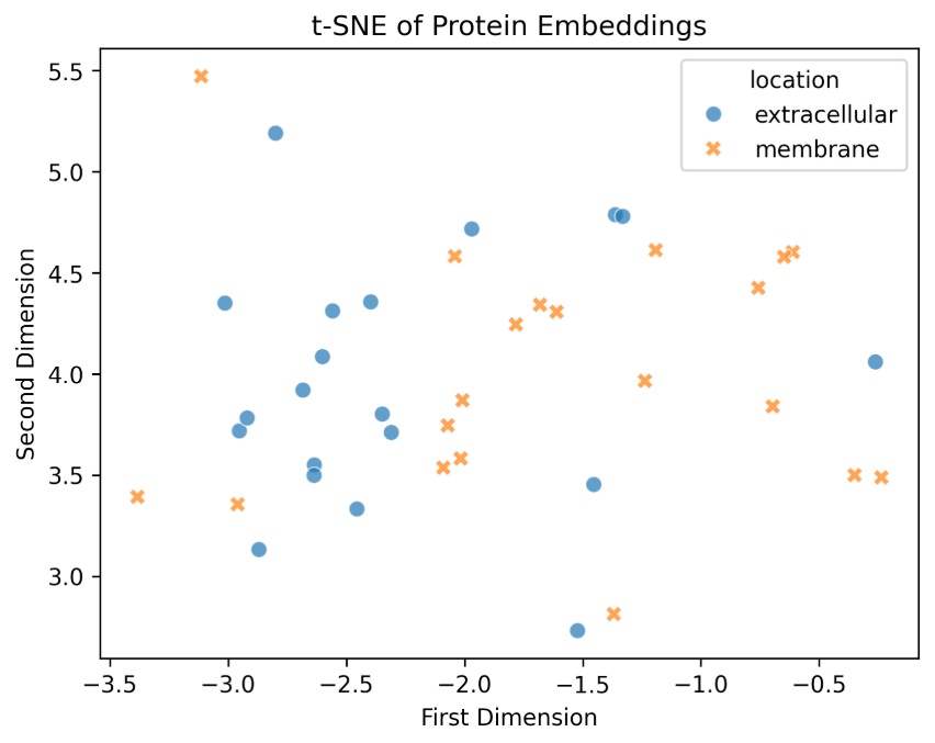
Now, we'll see an interesting example of protein embeddings: the difference between proteins from different cellular locations.
To give a concrete example, let's see these two protein categories:
Extracellular(GO:0005576): proteins secreted outside the cell, often involved in signaling, immune response, or structural rolesMembrane(GO:0016020): proteins embedded in or associated with cell membranes, frequently functioning in transport, signaling, or cell–cell interaction
Certain types of proteins have characteristic sequence features that correlate with where they function in the cell - structural features are encoded into protein sequences.
So, the question is: Are these structural features reflected in the learned embeddings?
Let's start by getting familiar with the data.
import pandas as pd

from dlfb.utils.context import assets

protein_df = pd.read_csv(assets("proteins/datasets/sequence_df_cco.csv"))
protein_df = protein_df[~protein_df["term"].isin(["GO:0005575", "GO:0110165"])]
num_proteins = protein_df["EntryID"].nunique()

#        EntryID             Sequence  taxonomyID        term aspect  Length
# 0       O95231  MRLSSSPPRGPQQLSS...        9606  GO:0005622    CCO     258
# 1       O95231  MRLSSSPPRGPQQLSS...        9606  GO:0031981    CCO     258
# 2       O95231  MRLSSSPPRGPQQLSS...        9606  GO:0043229    CCO     258
# ...        ...                  ...         ...         ...    ...     ...
# 337551  E7ER32  MPPLKSPAAFHEQRRS...        9606  GO:0031974    CCO     798
# 337552  E7ER32  MPPLKSPAAFHEQRRS...        9606  GO:0005634    CCO     798
# 337553  E7ER32  MPPLKSPAAFHEQRRS...        9606  GO:0005654    CCO     798
With this dataset, we want to filter only the sequences from the extracellular and membrane groups. And then, we separate and categorize them into their own list.
num_locations = protein_df.groupby("EntryID")["term"].nunique()
proteins_one_location = num_locations[num_locations == 1].index
protein_df = protein_df[protein_df["EntryID"].isin(proteins_one_location)]

go_function_examples = {
  "extracellular": "GO:0005576",
  "membrane": "GO:0016020",
}

sequences_by_function = {}

min_length = 100
max_length = 500
num_samples = 20

for function, go_term in go_function_examples.items():
  proteins_with_function = protein_df[
    (protein_df["term"] == go_term)
    & (protein_df["Length"] >= min_length)
    & (protein_df["Length"] <= max_length)
  ]
  print(
    f"Found {len(proteins_with_function)} human proteins\n"
    f"with the molecular function '{function}' ({go_term}),\n"
    f"and {min_length}<=length<={max_length}.\n"
    f"Sampling {num_samples} proteins at random.\n"
  )
  sequences = list(
    proteins_with_function.sample(num_samples, random_state=42)["Sequence"]
  )
  sequences_by_function[function] = sequences

# Found 164 human proteins
# with the molecular function 'extracellular' (GO:0005576),
# and 100<=length<=500.
# Sampling 20 proteins at random.

# Found 65 human proteins
# with the molecular function 'membrane' (GO:0016020),
# and 100<=length<=500.
# Sampling 20 proteins at random.
With the sequences in hand, we can tokenize and pass them to the model to extract their embeddings using the ESM2 model.
Before doing that, let's create this function called get_mean_embeddings to abstract how we get the embedding for an entire protein.
def get_mean_embeddings(
  sequences: list[str],
  tokenizer: PreTrainedTokenizer,
  model: PreTrainedModel,
  device: torch.device | None = None,
) -> np.ndarray:
  if not device:
    device = get_device()

  model_inputs = tokenizer(sequences, padding=True, return_tensors="pt")
  model_inputs = {k: v.to(device) for k, v in model_inputs.items()}
  model = model.to(device)
  model.eval()

  with torch.no_grad():
    outputs = model(**model_inputs)
    mean_embeddings = outputs.last_hidden_state.mean(dim=1)

  return mean_embeddings.detach().cpu().numpy()
For this function, we can see that we start with the input tokenization that will be used as input for the model. Then, we get the output of the model, the last hidden state, and compute the mean pooling, using last_hidden_state and mean methods.
And finally returns the protein embeddings.
With the sequences_by_function and the get_mean_embeddings, we get the protein embeddings for each protein.
protein_embeddings = {
  loc: get_mean_embeddings(sequences_by_function[loc], tokenizer, model)
  for loc in ["extracellular", "membrane"]
}

labels, embeddings = [], []

for location, embedding in protein_embeddings.items():
  labels.extend([location] * embedding.shape[0])
  embeddings.append(embedding)
To better visualize these embeddings, let's parse them into a 2-dimensional dataframe using TSNE:
import numpy as np
import seaborn as sns
from sklearn.manifold import TSNE

embeddings_tsne = TSNE(n_components=2, random_state=42).fit_transform(
  np.vstack(embeddings)
)
embeddings_tsne_df = pd.DataFrame(
  {
    "first_dimension": embeddings_tsne[:, 0],
    "second_dimension": embeddings_tsne[:, 1],
    "location": np.array(labels),
  }
)
And then, we plot the embeddings:
fig = sns.scatterplot(
  data=embeddings_tsne_df,
  x="first_dimension",
  y="second_dimension",
  hue="location",
  style="location",
  s=50,
  alpha=0.7,
)
plt.title("t-SNE of Protein Embeddings")
fig.set_xlabel("First Dimension")
fig.set_ylabel("Second Dimension");
They are grouped, meaning the embeddings are learning protein locations through only the sequences. This suggests that the learned embeddings reflect biologically meaningful patterns—even without any explicit supervision for cellular location.
Predicting Protein Function
Before working on the prediction model, let's build the dataset. This is an interesting section because it covers the reality and one of the most important parts of ML projects: Data Pre-Processing.
There are separate datasets that we will glue together through an identifier. First, we get the labels, merge them with the GO descriptions, then merge with the sequences from a fasta file, and finally merge with the taxonomy data.
Here's the labels:
labels
#             EntryID        term aspect
# 0        A0A009IHW8  GO:0008152    BPO
# 1        A0A009IHW8  GO:0034655    BPO
# 2        A0A009IHW8  GO:0072523    BPO
# ...             ...         ...    ...
# 5363860      X5M5N0  GO:0005515    MFO
# 5363861      X5M5N0  GO:0005488    MFO
# 5363862      X5M5N0  GO:0003674    MFO
Then, we have the GO terms with their respective descriptions:
go_term_descriptions
#              term          description
# 0      GO:0000001  mitochondrion in...
# 1      GO:0000002  mitochondrial ge...
# 2      GO:0000006  high-affinity zi...
# ...           ...                  ...
# 40211  GO:2001315  UDP-4-deoxy-4-fo...
# 40212  GO:2001316  kojic acid metab...
# 40213  GO:2001317  kojic acid biosy...
This is the first merge we do: labels and description via the term ‘identifier’.
labels = labels.merge(go_term_descriptions, on="term")
labels
#             EntryID        term aspect          description
# 0        A0A009IHW8  GO:0008152    BPO    metabolic process
# 1        A0A009IHW8  GO:0034655    BPO  nucleobase-conta...
# 2        A0A009IHW8  GO:0072523    BPO  purine-containin...
# ...             ...         ...    ...                  ...
# 4933955      X5M5N0  GO:0005515    MFO      protein binding
# 4933956      X5M5N0  GO:0005488    MFO              binding
# 4933957      X5M5N0  GO:0003674    MFO   molecular_function
The sequence data comes in this format:
sequence_df
#            EntryID             Sequence  Length
# 0           P20536  MNSVTVSHAPYTITYH...     218
# 1           O73864  MTEYRNFLLLFITSLS...     354
# 2           O95231  MRLSSSPPRGPQQLSS...     258
# ...            ...                  ...     ...
# 142243      Q5RGB0  MADKGPILTSVIIFYL...     448
# 142244  A0A2R8QMZ5  MGRKKIQITRIMDERN...     459
# 142245  A0A8I6GHU0  HCISSLKLTAFFKRSF...     138
And this is the taxonomy:
taxonomy
#            EntryID  taxonomyID
# 0           Q8IXT2        9606
# 1           Q04418      559292
# 2           A8DYA3        7227
# ...            ...         ...
# 142243  A0A2R8QBB1        7955
# 142244      P0CT72      284812
# 142245      Q9NZ43        9606
We can merge the sequences with the taxonomy through the EntryID:
sequence_df = sequence_df.merge(taxonomy, on="EntryID")
Before moving on, let's filter only the sequences from humans (human proteins). This means we only want the 9606 taxonomy IDs:
sequence_df = sequence_df[sequence_df["taxonomyID"] == 9606]
Then, we finally merge the sequence with the labels:
sequence_df = sequence_df.merge(labels, on="EntryID")
sequence_df
#        EntryID             Sequence  Length  taxonomyID        term aspect  description
# 0       O95231  MRLSSSPPRGPQQLSS...     258        9606  GO:0003676    MFO  nucleic acid bin...
# 1       O95231  MRLSSSPPRGPQQLSS...     258        9606  GO:1990837    MFO  sequence-specifi...
# 2       O95231  MRLSSSPPRGPQQLSS...     258        9606  GO:0001216    MFO  DNA-binding tran...
# ...        ...                  ...     ...         ...         ...    ...  ...
# 152523  Q86TI6  MGAAAVRWHLCVLLAL...     347        9606  GO:0005515    MFO  protein binding
# 152524  Q86TI6  MGAAAVRWHLCVLLAL...     347        9606  GO:0005488    MFO  binding
# 152525  Q86TI6  MGAAAVRWHLCVLLAL...     347        9606  GO:0003674    MFO  molecular_function
After gluing everything together, we need to process it to make it ready to train the model.
# Filtering out the ‘uninteresting’, generic functions
uninteresting_functions = [
  "GO:0003674",  # "molecular function". Applies to 100% of proteins.
  "GO:0005488",  # "binding". Applies to 93% of proteins.
  "GO:0005515",  # "protein binding". Applies to 89% of proteins.
]

sequence_df = sequence_df[~sequence_df["term"].isin(uninteresting_functions)]

# Filtering out the rare labels (only labels with more than or equal to 50 sequences)
common_functions = (
  sequence_df["term"]
  .value_counts()[sequence_df["term"].value_counts() >= 50]
  .index
)

sequence_df = sequence_df[sequence_df["term"].isin(common_functions)]

# Reshape the dataframe, so each row has a protein, and each term is transformed into columns
sequence_df = (
  sequence_df[["EntryID", "Sequence", "Length", "term"]]
  .assign(value=1)
  .pivot(
    index=["EntryID", "Sequence", "Length"], columns="term", values="value"
  )
  .fillna(0)
  .astype(int)
  .reset_index()
)
This is what's happening here:
- Filtering out the ‘uninteresting’, generic functions
- Filtering out the rare labels (only labels with more than or equal to 50 sequences)
- Reshape the dataframe, so each row has a protein, and each term is transformed into columns
Here's the entire dataframe now:
sequence_df
# term      EntryID             Sequence  Length  GO:0000166  GO:0000287  ...  GO:1901702  GO:1901981  GO:1902936  GO:1990782  GO:1990837
# 0      A0A024R6B2  MIASCLCYLLLPATRL...     670           0           0  ...  0           0           0           0           0
# 1      A0A087WUI6  MSRKISKESKKVNISS...     698           0           0  ...  0           0           0           0           0
# 2      A0A087X1C5  MGLEALVPLAMIVAIF...     515           0           0  ...  0           0           0           0           0
# ...           ...                  ...     ...         ...         ...  ...  ...         ...         ...         ...         ...
# 10706      Q9Y6Z7  MNGFASLLRRNQFILL...     277           0           0  ...  0           0           0           0           0
# 10707      X5D778  MPKGGCPKAPQQEELP...     421           0           0  ...  0           0           0           0           0
# 10708      X5D7E3  MLDLTSRGQVGTSRRM...     237           0           0  ...  0           0           0           0           0
Great! We have the data, and now we can work on splitting it into training, validation, and test sets for the model training and evaluation.
As the book states, this is what each one of them will be used for further:
Training set: Used to fit the model. The model sees this data during training and uses it to learn patterns.Validation set: Used to evaluate the model’s performance during development. We use this to tune hyperparameters and compare model variants.Test set: Used only once, for final evaluation. Crucially, we avoid using this data to guide model design decisions. It serves as our best estimate of how well the model would generalize to completely unseen data.
We have 60% used for training, 20% for validation, and 20% for testing:
from sklearn.model_selection import train_test_split

train_sequence_ids, valid_test_sequence_ids = train_test_split(
  list(set(sequence_df["EntryID"])), test_size=0.40, random_state=42
)

valid_sequence_ids, test_sequence_ids = train_test_split(
  valid_test_sequence_ids, test_size=0.50, random_state=42
)

sequence_splits = {
  "train": sequence_df[sequence_df["EntryID"].isin(train_sequence_ids)],
  "valid": sequence_df[sequence_df["EntryID"].isin(valid_sequence_ids)],
  "test": sequence_df[sequence_df["EntryID"].isin(test_sequence_ids)],
}
Let's validate each of them and check if they have an accurate number of examples:
for split, df in sequence_splits.items():
  print(f"{split} has {len(df)} entries.")

# train has 3574 entries.
# valid has 1191 entries.
# test has 1192 entries.
Extracting Embeddings for Protein Examples
Now that we have each data set, we can start using the pretrained model to get the embeddings. These embeddings will be glued into each data set and transformed into additional columns. We'll see that they will be labeled with the ME prefix, from 1 to 640, e.g., ME:1 … ME:640.
import torch

def get_device() -> torch.device:
  return torch.device("cuda" if torch.cuda.is_available() else "cpu")

model_checkpoint = "facebook/esm2_t30_150M_UR50D"
tokenizer = AutoTokenizer.from_pretrained(model_checkpoint)
model = EsmModel.from_pretrained(model_checkpoint)
n_batches = ceil(sequence_df.shape[0] / batch_size)
batches: list[np.ndarray] = []

for i in range(n_batches):
  batch_seqs = list(
    sequence_df["Sequence"][i * batch_size : (i + 1) * batch_size]
  )
  batches.extend(get_mean_embeddings(batch_seqs, tokenizer, model, device))

embeddings = pd.DataFrame(np.vstack(batches))
embeddings.columns = [f"ME:{int(i)+1}" for i in range(embeddings.shape[1])]
df = pd.concat([sequence_df.reset_index(drop=True), embeddings], axis=1)
Because running on this pretrained model takes time, we can use GPUs together with batch iterations for parallel processing. But the essential part of this code is the part where we pass the batch sequences to the get_mean_embeddings function to the embeddings, and then concatenate that to the dataframe.
Again, this function will get the mean-pooled hidden states from the final layer of the ESM2 model, and these embeddings capture biochemical and structural information.
This is what we have after getting the embeddings and concatenating them to the dataframe:
         EntryID             Sequence  Length  GO:0000166  GO:0000287  ...  ME:636    ME:637    ME:638    ME:639    ME:640
0     A0A0C4DG62  MAHVGSRKRSRSRSRS...     218           0           0  ...  0.062926  0.040286  0.030008 -0.033614  0.023891
1     A0A1B0GTB2  MVITSENDEDRGGQEK...      48           0           0  ...  0.129815 -0.044294  0.023842 -0.020635  0.125583
2         A0AVI4  MDSPEVTFTLAYLVFA...     362           0           0  ...  0.153848 -0.075747  0.024440 -0.123321  0.020945
...          ...                  ...     ...         ...         ...  ...       ...       ...       ...       ...       ...
3571      Q9Y6W5  MPLVTRNIEPRHLCRQ...     498           0           0  ...  -0.001535 -0.084161 -0.014317 -0.141801 -0.040719
3572      Q9Y6W6  MPPSPLDDRVVVALSR...     482           0           0  ...  0.120192 -0.086032 -0.016481 -0.108710 -0.077937
3573      Q9Y6Y9  MLPFLFFSTLFSSIFT...     160           0           0  ...  0.114847 -0.028570  0.084638  0.038610  0.087047
Now we have the identification, the sequence, the sequence length, the labels (protein functions as targets), and the embeddings. The labels start with the prefix GO and the embeddings with ME.
Because we have terms in the dataframe and the actual label is defined with value 1 (and 0 for when it's not the actual term), the GO labels are represented as a one-hot encoding.
Before moving on, let's abstract that code into a function:
def get_sequence_embeddings(
  sequence_df: pd.DataFrame,
  tokenizer: PreTrainedTokenizer,
  model: PreTrainedModel,
  batch_size: int = 64,
) -> None:
  device = get_device()
  n_batches = ceil(sequence_df.shape[0] / batch_size)
  batches: list[np.ndarray] = []

  for i in range(n_batches):
    batch_seqs = list(
      sequence_df["Sequence"][i * batch_size : (i + 1) * batch_size]
    )
    batches.extend(get_mean_embeddings(batch_seqs, tokenizer, model, device))

  embeddings = pd.DataFrame(np.vstack(batches))
  embeddings.columns = [f"ME:{int(i)+1}" for i in range(embeddings.shape[1])]

  return pd.concat([sequence_df.reset_index(drop=True), embeddings], axis=1)
Then, we will convert it into a dataset using TensorFlow. Basically, a dataset of an embedding and the target.
import tensorflow as tf

def convert_to_tfds(
  df: pd.DataFrame,
  embeddings_prefix: str = "ME:",
  target_prefix: str = "GO:",
  is_training: bool = False,
  shuffle_buffer: int = 50,
) -> tf.data.Dataset:
  dataset = tf.data.Dataset.from_tensor_slices(
    {
      "embedding": df.filter(regex=f"^{embeddings_prefix}").to_numpy(),
      "target": df.filter(regex=f"^{target_prefix}").to_numpy(),
    }
  )
  if is_training:
    dataset = dataset.shuffle(shuffle_buffer).repeat()

  return dataset
Putting everything together, we create this build_dataset function:
model_checkpoint = "facebook/esm2_t30_150M_UR50D"
tokenizer = AutoTokenizer.from_pretrained(model_checkpoint)
model = EsmModel.from_pretrained(model_checkpoint)

def build_dataset() -> dict[str, tf.data.Dataset]:
  dataset_splits = {}

  for split, df in sequence_splits.items():
    dataset_splits[split] = convert_to_tfds(
      df=get_sequence_embeddings(
        sequence_df=df,
        tokenizer=tokenizer,
        model=model,
      ),
      is_training=(split == "train"),
    )

  return dataset_splits
It goes through the data splits, gets the sequence embeddings, passes them to the convert_to_tfds function, and store each dataset split into the dataset_splits object.
dataset_splits = build_dataset()
This will hold all the datasets for each split (train, validation, and test).
Now we are ready to train the model.
Training the Model
Before starting training the model, let's recap what our goal is. Based on the protein embeddings (extracted meaning from protein sequences), our goal is to predict which protein function is the actual one among all the 303 molecular functions.
A protein sequence can be associated with multiple functions at the same time. This is, by definition, a multi-label classification problem.
First, we build a simple model
import flax.linen as nn
from flax.training import train_state

class Model(nn.Module):
  num_targets: int
  dim: int = 256

  @nn.compact
  def __call__(self, x):
    x = nn.Sequential(
      [
        nn.Dense(self.dim * 2),
        jax.nn.gelu,
        nn.Dense(self.dim),
        jax.nn.gelu,
        nn.Dense(self.num_targets),
      ]
    )(x)
    return x

  def create_train_state(self, rng: jax.Array, dummy_input, tx) -> TrainState:
    variables = self.init(rng, dummy_input)
    return TrainState.create(
      apply_fn=self.apply, params=variables["params"], tx=tx
    )
This model implements just a sequential layer of Dense and gelu activation function, finishing with a dense layer projecting to the number of function labels (the number of targets or labels — the output is represented by logits, not probabilities).
It will use the pretrained embeddings as input and only update the model parameters without updating the pretrained model parameters. This means that the model is frozen on top of the ESM2 embeddings.
Let's instantiate the model:
targets = list(train_df.columns[train_df.columns.str.contains("GO:")])
mlp = Model(num_targets=len(targets))
In the training loop, we need to do a forward pass, compute the loss, calculate gradients, and update the model parameters using those gradients. Let's build this training step:
@jax.jit
def train_step(state, batch):
  def calculate_loss(params):
    logits = state.apply_fn({"params": params}, x=batch["embedding"])
    # multi-label classification loss
    loss = optax.sigmoid_binary_cross_entropy(logits, batch["target"]).mean()
    return loss

  grad_fn = jax.value_and_grad(calculate_loss, has_aux=False)
  loss, grads = grad_fn(state.params)
  # update the gradients
  state = state.apply_gradients(grads=grads)
  return state, loss
We use an appropriate way to compute the loss for a multi-label classification problem, a combination of a sigmoid activation and binary cross-entropy loss. This will compute a yes/no answer for each molecular function (label) independently, because it can have many functions simultaneously.
The value_and_grad function evaluates the calculate_loss and its gradients. We then use these gradients to update the model's weight parameters.
To complete the model, we need to evaluate its performance based on metrics.
Here are the metrics we will calculate (book definition):
Accuracy: The fraction of correct predictions across all labels. In multilabel classification with imbalanced data (like this), accuracy can be misleading—most labels are zero, so a model that always predicts “no function” would appear accurate. Still, it’s an intuitive metric and we’ll include it for now.Recall: The proportion of actual function labels the model correctly predicted (i.e., true positives/all actual positives). High recall means the model doesn’t miss many true functions.Precision: The proportion of predicted function labels that are correct (i.e., true positives/all predicted positives). High precision means the model avoids false alarms.Area under the precision-recall curve (auPRC): Summarizes the tradeoff between precision and recall at different thresholds. Particularly useful in highly imbalanced settings like this one.Area under the receiver operating characteristic curve (auROC): Measures the model’s ability to distinguish positive from negative examples across all thresholds. While it’s a standard metric of discrimination ability, it can sometimes be misleading in highly imbalanced datasets, as it gives equal weight to both classes.
The calculation will follow this idea:
- Apply sigmoid to the logits to get function probabilities.
- Threshold those probabilities (e.g., at 0.5) to get binary predictions.
> 0.5: predict to be that function< 0.5: predict not to be that function
- Compare these to the true function labels to compute metrics like accuracy, precision, recall, auPRC, and auROC.
Here's the implementation:
import sklearn

def compute_metrics(
  targets: np.ndarray, probs: np.ndarray, thresh=0.5
) -> dict[str, float]:
  if np.sum(targets) == 0:
    return {
      m: 0.0 for m in ["accuracy", "recall", "precision", "auprc", "auroc"]
    }

  return {
    "accuracy": metrics.accuracy_score(targets, probs >= thresh),
    "recall": metrics.recall_score(targets, probs >= thresh).item(),
    "precision": metrics.precision_score(
      targets,
      probs >= thresh,
      zero_division=0.0,
    ).item(),
    "auprc": metrics.average_precision_score(targets, probs).item(),
    "auroc": metrics.roc_auc_score(targets, probs).item(),
  }
With this function, we can calculate the metrics for each target. We just need the targets and the probabilities and pass them to this function. Let's build a calculate_per_target_metrics function to handle that:
def calculate_per_target_metrics(logits, targets):
  probs = jax.nn.sigmoid(logits)
  target_metrics = []

  for target, prob in zip(targets, probs):
    target_metrics.append(compute_metrics(target, prob))

  return target_metrics
And then, we put everything together on the evaluation step:
def eval_step(state, batch) -> dict[str, float]:
  logits = state.apply_fn({"params": state.params}, x=batch["embedding"])
  loss = optax.sigmoid_binary_cross_entropy(logits, batch["target"]).mean()
  target_metrics = calculate_per_target_metrics(logits, batch["target"])
  metrics = {
    "loss": loss.item(),
    **pd.DataFrame(target_metrics).mean(axis=0).to_dict(),
  }
  return metrics
We are basically computing the metrics for each protein in the batch and then computing the average of those metrics. This will be used for the validation set.
All the training, the metrics computation, and the evaluation step come together on the train function.
The function trains the model in batches for the train set, and for every 30 steps, the model is evaluated on a validation set batch, and it calculates the performance metrics.
In the end, we have train and validation metrics:
def train(
  state: TrainState,
  dataset_splits: dict[str, tf.data.Dataset],
  batch_size: int,
  num_steps: int = 300,
  eval_every: int = 30,
):
  train_metrics, valid_metrics = [], []
  train_batches = (
    dataset_splits["train"]
    .batch(batch_size, drop_remainder=True)
    .as_numpy_iterator()
  )

  steps = tqdm(range(num_steps))

  for step in steps:
    steps.set_description(f"Step {step + 1}")
    state, loss = train_step(state, next(train_batches))
    train_metrics.append({"step": step, "loss": loss.item()})

    if step % eval_every == 0:
      eval_metrics = []

      for eval_batch in (
        dataset_splits["valid"].batch(batch_size=batch_size).as_numpy_iterator()
      ):
        eval_metrics.append(eval_step(state, eval_batch))

      valid_metrics.append(
        {"step": step, **pd.DataFrame(eval_metrics).mean(axis=0).to_dict()}
      )

  return state, {"train": train_metrics, "valid": valid_metrics}
We compute the metrics for each target and calculate the mean for steps and batches.
- The average is calculated for all metrics for each protein sequence/target
- We summarize the model performance based on the average of each metric
A simple example is like this:
target_metrics = [
    # Metrics for target A
    {"accuracy": 0.9, "recall": 0.8, "precision": 0.85, "auprc": 0.92, "auroc": 0.95},
    # Metrics for target B
    {"accuracy": 0.85, "recall": 0.75, "precision": 0.8, "auprc": 0.88, "auroc": 0.91}
]

# ======

pd.DataFrame(target_metrics)

    accuracy  recall  precision  auprc  auroc
0      0.90    0.80       0.85   0.92   0.95
1      0.85    0.75       0.80   0.88   0.91

# ======

pd.DataFrame(target_metrics).mean(axis=0)

accuracy     0.875
recall       0.775
precision    0.825
auprc        0.900
auroc        0.930
dtype: float64
Evaluating the Model
Now that we have everything in place, we can start training the model on the dataset and then evaluate the metrics.
rng = jax.random.PRNGKey(42)
rng, rng_init = jax.random.split(key=rng, num=2)

state, metrics = train(
  state=mlp.create_train_state(
    rng=rng_init, dummy_input=batch["embedding"], tx=optax.adam(0.001)
  ),
  dataset_splits=dataset_splits,
  batch_size=32,
  num_steps=300,
  eval_every=30,
)
With those metrics, we can plot them:
import matplotlib.pyplot as plt
import seaborn as sns

NAMED_COLORS = OrderedDict(
  [
    ("red", "#e41a1c"),
    ("blue", "#377eb8"),
    ("green", "#4daf4a"),
    ("purple", "#984ea3"),
    ("orange", "#ff7f00"),
    ("yellow", "#ffff33"),
    ("brown", "#a65628"),
    ("pink", "#f781bf"),
    ("gray", "#999999"),
  ]
)

DEFAULT_SPLIT_COLORS = {
  "train": NAMED_COLORS["blue"],
  "valid": NAMED_COLORS["green"],
  "test": NAMED_COLORS["orange"],
}

fig, ax = plt.subplots(nrows=1, ncols=2, figsize=(9, 4))

learning_data = pd.concat(
  pd.DataFrame(metrics[split]).melt("step").assign(split=split)
  for split in ["train", "valid"]
)

sns.lineplot(
  ax=ax[0],
  x="step",
  y="value",
  hue="split",
  data=learning_data[learning_data["variable"] == "loss"],
  palette=DEFAULT_SPLIT_COLORS,
)
ax[0].set_title("Loss over training steps.")

sns.lineplot(
  ax=ax[1],
  x="step",
  y="value",
  hue="variable",
  style="variable",
  data=learning_data[learning_data["variable"] != "loss"],
  palette="Set2",
)
plt.legend(loc="center left", bbox_to_anchor=(1, 0.5))
ax[1].set_title("Validation metrics over training steps.");
It plots two graphs: one for the loss over the training and validation steps, and another for the validation metrics over the training steps.
Comparing the validation and the test set is also a good check.
eval_metrics = []

for split in ["valid", "test"]:
  split_metrics = []

  for eval_batch in dataset_splits[split].batch(32).as_numpy_iterator():
    split_metrics.append(eval_step(state, eval_batch))

  eval_metrics.append(
    {"split": split, **pd.DataFrame(split_metrics).mean(axis=0).to_dict()}
  )

pd.DataFrame(eval_metrics)
#    split      loss  accuracy    recall  precision     auprc     auroc
# 0  valid  0.080156  0.978457  0.126869   0.418515  0.411870  0.880883
# 1   test  0.080675  0.978032  0.125820   0.435193  0.410439  0.879234
The test set metrics closely mirror those observed on the validation set, which is good.
With that, we end this first post of the series of reading, learning, and applying the knowledge from the book. This first chapter talked about a bunch of stuff, and I learned a ton about biology, proteins, bio data, and ML for these kinds of problems.